Chapter 14 Hypothesis Testing on Whole Models

A wise man … proportions his belief to the evidence. – David Hume (1711 – 1776), Scottish philosopher

Fitted models describe patterns in samples. Modelers interpret these patterns as indicating relationships between variables in the population from which the sample was drawn. But there is another possibility. Just as the constellations in the night sky are the product of human imagination applied to the random scattering of stars within range of sight, so the patterns indicated by a model might be the result of accidental alignments in the sample.

Deciding how seriously to take the patterns identified by a model is a problem that involves judgment. Are the patterns consistent with well established understanding of how the system works? Are the patterns corroborated by other sources of data? Are the model results sensitive to trivial changes in the model design?

Before undertaking that judgment, it helps to apply a much simpler standard of evidence. The conventional interpretation of a model such as A ~ B + C + … is that the variables on the right side of the modeler’s tilde explain the response variable on the left side. The first question to ask is whether the explanation provided by the model is stronger than the “explanation” that would be arrived at if the variables on the right side were random – explanatory variables in name only without any real connection with the response variable A.

It’s important to remember that in a hypothesis test, the null hypothesis is about the population. The null hypothesis claims that in the population the explanatory variables are unlinked to the response variable. Such a hypothesis does not rule out the possibility that, in the sample, the explanatory variables are aligned with the response variable. The hypothesis merely claims that any such alignment is accidental, due to the randomness of the sampling process.

14.1 The Permutation Test

The null hypothesis is that the explanatory variables are unlinked with the response variable. One way to see how big a test statistic will be in a world where the null hypothesis holds true is to randomize the explanatory variables in the sample to destroy any relationship between them and the response variable. To illustrate how this can be done in a way that stays true to the sample, consider a small data set:

A	B	C
3	37.1	M
4	17.4	M
5	26.8	F
7	44.3	F
5	19.7	F

Imagine that the table has been cut into horizontal slips with one case on each slip. The response variable – say, A – has been written to the left of a dotted line. The explanatory variables B and C are on the right of the dotted line, like this:

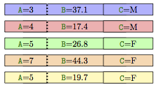
To randomize the cases, tear each sheet along the dotted line. Place the right sides – the explanatory variables – on a table in their original order. Then, randomly shuffle the left halves – the response variable – and attach each to a right half.

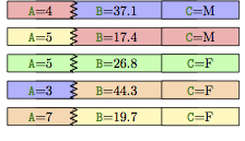
None of the cases in the shuffle are genuine cases, except possibly by chance. Yet each of the shuffled explanatory variables is true to its distribution in the original sample and the relationships among explanatory variables – collinearity and multi-collinearity – are also authentic.

Each possible order for the left halves of the cards is called a permutation. A hypothesis test conducted in this way is called a permutation test.

The logic of a permutation test is straightforward. To set up the test, you need to choose a test statistic that reflects some aspect of the system of interest to you.

Here are the steps involved in permutation test:

• Step 1. Calculate the value of the test statistic on the original data.
  
• Step 2. Permute the data and calculate the test statistic again. Repeat this many times, collecting the results. This gives the distribution of the test statistic under the null hypothesis.
  
• Step 3. Read off the p-value as the fraction of the results in (2) that are more extreme than the value in (1).

To illustrate, consider a model of heights from Galton’s data and a question Galton didn’t consider: Does the number of children in a family help explain the eventual adult height of the children? Perhaps in families with large numbers of children, there is competition over food, so children don’t grow so well. Or, perhaps having a large number of children is a sign of economic success, and the children of successful families have more to eat.

The regression report indicates that larger family size is associated with shorter children:

	Estimate	Std. Error	t-value	p-value
Intercept	67.800	0.296	228.96	0.0000
nkids	-0.169	0.044	-3.83	0.0001

For every additional sibling, the family’s children are shorter by about 0.17 inches on average. The confidence interval is −0.169 ± 0.088.

Now for the permutation test, using the coefficient on nkids as the test statistic:

• Step 1 Calculate the test statistic on the data without any shuffling. As shown above, the coefficient on is −0.169.
  
• Step 2. Permute and re-calculate the test statistic, many times. One set of 10000 trials gave values of −0.040, 0.037, −0.094, −0.069, 0.062, −0.045, and so on. The distribution is shown in Figure 14.1.
• Step 3. The p-value is fraction of times that the values from (2) are more extreme than the value of −0.169 from the unshuffled data. As Figure 14.1 shows, few of the permutations produced an nkid coefficient anywhere near −0.169. The p-value is very small, p< 0.001.

Conclusion, the number of kids in a family accounts for somewhat more of the children’s heights than is likely to occur with a random explanatory variable.

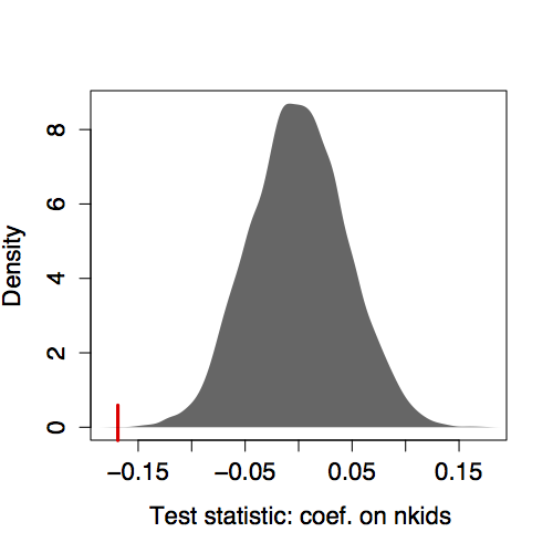
Figure 14.1: Distribution of the coefficient on nkids from the model height ~ 1+nkids from many permutation trials. Tick mark: the coefficient -0.169 from the unshuffled data.

The idea of a permutation test is almost a century old. It was proposed originally by statistician Ronald Fisher (1890-1960). Permutation tests were infeasible for even moderately sized data sets until the 1970s when inexpensive computation became a reality. In Fisher’s day, when computing was expensive, permutation tests were treated as a theoretical notion and actual calculations were performed using algebraic formulas and calculus. Such formulas could be derived for a narrow range of test statistics such as the sample mean, differences between group means, and the coefficient of determination R². Fisher himself derived the sampling distributions of these test statistics.(Fisher 1924)

Figure 14.2: Sir Ronald Fisher

14.2 R² and the F Statistic

The coefficient of determination R² measures what fraction of the variance of the response variable is “explained” or “accounted for” or – to put it simply – “modeled” by the explanatory variables. R² is a comparison of two quantities: the variance of the fitted model values to the variance of the response variable. R² is a single number that puts the explanation in the context of what remains unexplained. It’s a good test statistic for a hypothesis test.

Using R² as the test statistic in a permutation test would be simple enough. There are advantages, however, to thinking about things in terms of a closely related statistic invented by Fisher and named in honor of him: the F statistic.

Like R², the F statistic compares the size of the fitted model values to the size of the residuals. But the notion of “size” is somewhat different. Rather than measuring size directly by the variance or by the sum of squares, the F statistic takes into account the number of model vectors.

To see where F comes from, consider the random model walk . In a regular random walk, each new step is taken in a random direction. In a random model walk, each “step” consists of adding a new random explanatory term to a model. The “position” is measured as the R² from the model.

The starting point of the random model walk is the simple model A ~ 1 with just m=1 model vector. This model always produces R² = 0 because the all-cases-the-same model can’t account for any variance. Taking a “step” means adding a random model vector, x₁, giving the model A ~ 1+x₁. Each new step adds a new random vector to the model:

m	Model
1	A ~ 1
2	A ~ 1+x₁
3	A ~ 1+x₁+x₂
4	A ~ 1+x₁+x₂+x₃
⋮
n	A ~ 1+x₁+x₂+x₃ + … + x𝑛₋₁

Figure 14.3 shows R² versus m for several random model walks in data with n=50 cases. Each successive step adds in its own individual random explanatory term.

All the random walks start at R² = 0 for m=1. All of them reach R² = 1 when m=n. Adding any more vectors beyond m=n simply creates redundancy; R² = 1 is the best that can be done.

Notice that each step increases R² – none of the random walks goes down in value as m gets bigger.

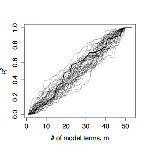
Figure 14.3: Random model walks for n=50 cases. The “position” of the walk is R². This is plotted versus number of model vectors m. The heavy line shows one simulation. The light lines show other simulations. All of the simulations reach R² = 1 when m=n.

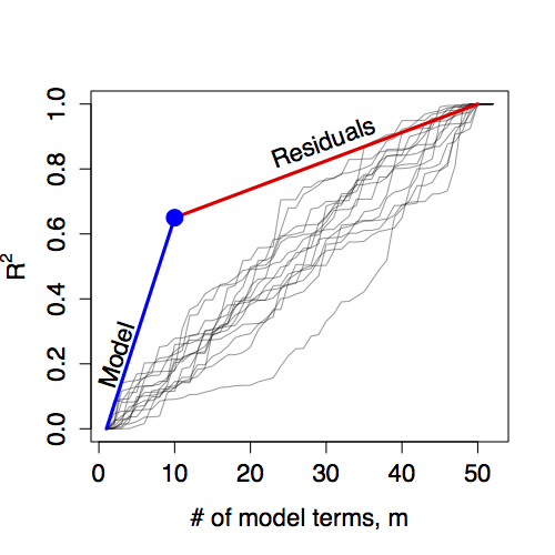
Figure 14.4: The R² from a fitted model defines a model walk with two segments. The F statistic is the ratio of the slopes of these segments. Here a model with m=10 has produced R² = 0.65 when fitted to a data set with n=50 cases.

The R² from a fitted model gives a single point on the model walk that divides the overall walk into two segments, as shown in Figure 14.4. The slope of each of the two segments has a straightforward interpretation. The slope of the segmented labeled “Model” describes the rate at which R² is increased by a typical model vector. The slope can be calculated as R² / (m−1).

The slope of the segment labeled “Residuals” describes how adding a random vector to the model would increase R². From the figure, you can see that a typical model vector increases R² much faster than a typical random vector. Numerically, the slope is (1−R²)/(m−n).

The F statistic is the ratio of these two slopes:

\(F = \frac{\mbox{slope of model segment}}{\mbox{slope of residual segment}} = \frac{R^2}{m-1} / \frac{1-R^2}{n-m}\) (14.1)

In interpreting the F statistic, keep in mind that if the model vectors were no better than random, F should be near 1. When F is much bigger than 1, it indicates that the model terms explain more than would be expected at random. The p-value provides an effective way to identify when F is “much bigger than 1.” Calculating the p-value involves knowing the exact shape of the F distribution. In practice, this is done with software.

The number m-1 in the numerator of F counts how many model terms there are other than the intercept. In standard statistical nomenclature, this is called the degrees of freedom of the numerator . The number n−m in the denominator of F counts how many random terms would need to be added to make a “perfect” fit to the response variable. This number is called the degrees of freedom of the denominator .

Example: Marriage and Astrology

Does your astrological sign predict when you will get married? To test this possibility, consider a small set of data collected from an on-line repository of marriage licenses in Mobile County, Alabama in the US. The licenses contain a variety of information: age at marriage, years of college, date of birth, date of the wedding and so on. For those with mystical interests, date of birth can be converted to an astrological sign, resulting in a data set that looks like this:

Sign	Age	College
Aquarius	22.6	4
Sagittarius	25.1	0
Taurus	39.6	1
Cancer	45.8	6
Leo	26.4	1

… and so on for 98 cases altogether.

There are, of course, 12 different astrological signs, so the model Age ~ Sign has m=12. With the intercept term, that leaves 11 vectors to represent Sign. Fitting the model produces R² = 0.070. To generate a p-value, this can be compared to the distribution of R² for random vectors with n=98 and m=12, giving p=0.885. This large value is consistent with the null hypothesis that Sign is unlinked with Age.

The pair m=12, R² = 0.070 gives one point on a model walk. This is compared to random model walks in the Figure 14.5. The 11 indicator vectors that arise from the 12 levels of Sign do not contribute more to R² than would be expected from 11 random vectors.

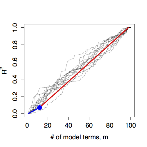
Figure 14.5: Random model walks compared to the model Age ~ Sign. The actual model does not stand out from the set of random model walks.

Now consider a different model, Age ~ College. This model undertakes to explain age at marriage by whether the person went to college. The R² from this model is only 0.065 – the College variable accounts for somewhat less of the variability in Age than astrological Sign. Yet this small R² is statistically significant – p=0.017. The reason is that College accomplishes its explanation using only a single model vector, compared to the 11 vectors in Sign. The model walk for the College model starts with a steep increase because the whole gain of 0.065 is accomplished with just one model vector, rather than being achieved using 11 vectors as in Sign.

14.3 The ANOVA Report

The F statistic compares the variation that is explained by the model to the variation that remains unexplained. Doing this involves taking apart the variation; partitioning it into a part associated with the model and a part associated with the residuals.

Such partitioning of variation is fundamental to statistical methods. When done in the context of linear models, this partitioning is given the name analysis of variance ANOVA for short. This name stays close to the dictionary definition of “analysis” as “the process of separating something into its constituent elements.” (“New Oxford American Dictionary” 2015)

The analysis of variance is often presented in a standard way: the ANOVA report . For example, here is the ANOVA report for the marriage-astrology model Age ~ Sign:

	Df	Sum Sq	Mean Sq	F value	p-value
Sign	11	1402	127	0.59	0.8359
Residuals	86	18724	218

There are two rows in this ANOVA report. The first refers to the explanatory variable, the second to the residual.

Since ANOVA is about variance, the mean of the response variable is subtracted out before the analysis is performed, just as it would be when calculating a variance. The column labeled “Sum Sq” gives the sum of squares of the fitted model values and the residual vector. The column headed “Df” is the degrees of freedom of the term. This is simply the number of model vectors associated with that term or, for the residual, the total number of cases minus the number of explanatory vectors. For a categorical variable, the number of explanatory vectors is the number of levels of that variable minus one for each redundant vector. (For instance, every categorical variable has one degree of redundancy with the intercept). Because there are 12 levels in Sign, the 12 astrological signs, the Sign variable has 11 degrees of freedom.

The degrees of freedom of the residuals is the number of cases n minus the number of model terms m.

Aside: F and R²

The R² doesn’t appear explicitly in the ANOVA report, but it’s easy to calculate since the report does give the square lengths of the two legs of the model triangle. In the above ANOVA report for Age ~ Sign, the square length of the hypotenuse is, through the pythagorean relationship, simply the sum of the two legs: in this report, 1402 + 18724 = 20126. The model’s R² is the square length of the fitted-model-value leg divided into the square length of the hypotenuse: 1402 / 20126 = 0.070.

The mean square in each row is the sum of squares divided by the degrees of freedom. The table’s F value is the ratio of the mean square of the fitted model values to the mean square of the residuals: 127 / 218 = 0.585 in this example. This is the same as given by Equation 14.1, but the calculations are being done in a different order.

Finally, the F value is converted to a p-value by look-up in the appropriate F distribution with the indicated degrees of freedom in the numerator and the denominator.

Example: Is height genetically determined?

Francis Galton’s study of height in the late 1800s was motivated by his desire to quantify genetic inheritance. In 1859, Galton read Charles Darwin’s On the Origin of Species in which Darwin first put forward the theory of natural selection of heritable traits. (Galton and Darwin were half-cousins, sharing the same grandfather, Erasmus Darwin.)

The publication of Origin of Species preceded by a half-century any real understanding of the mechanism of genetic heritability. Today, of course, even elementary-school children hear about DNA and chromosomes, but during Darwin’s life these ideas were unknown. Darwin himself thought that traits were transferred from the parents to the child literally through the blood, with individual traits carried by “gemmules.” Galton tried to confirm this experimentally by doing blood-mixing experiments on rabbits; these were unsuccessful at transferring traits.

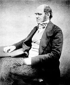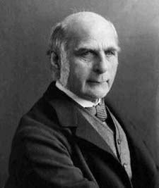Charles Darwin (1809-1882)	Francis Galton (1822-1911)

By collecting data on the heights of children and their parents, Galton sought to quantify to what extent height is determined genetically. Galton faced the challenge that the appropriate statistical methods had not yet been developed – he had to start down this path himself. In a very real sense, the development of ANOVA by Ronald Fisher in the early part of the twentieth century was a direct outgrowth of Galton’s work.

Had he been able to, here is the ANOVA report that Galton might have generated. The report summarizes the extent to which height is associated with inheritance from the mother and the father and by the genetic trait sex, using the model height ~ 1 + sex + mother + father.

	Df	Sum Sq	Mean Sq	F value	p-value
Genetic Terms	3	7366	2455	529	0.000
Residuals	894	4159	5

The F value is huge and accordingly the p-value is very small: the genetic variables are clearly explaining much more of height than random vectors.

If Galton had access to modern statistical approaches – even those from as long ago as the middle of the twentieth century – he might have wondered how to go further, for example how to figure out whether the mother and father each contribute to height, or whether it is a trait that comes primarily from one parent. Answering such questions involves partitioning the variance not merely between the model terms and the residual but among the individual model terms. This is the subject of Chapter 15.

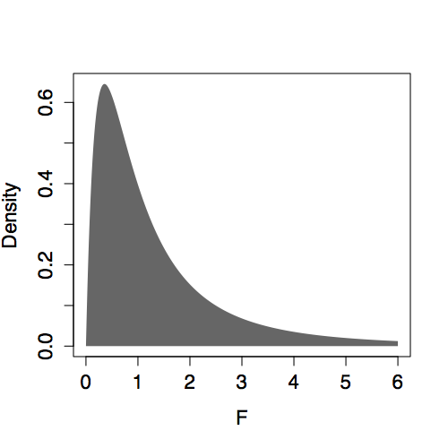
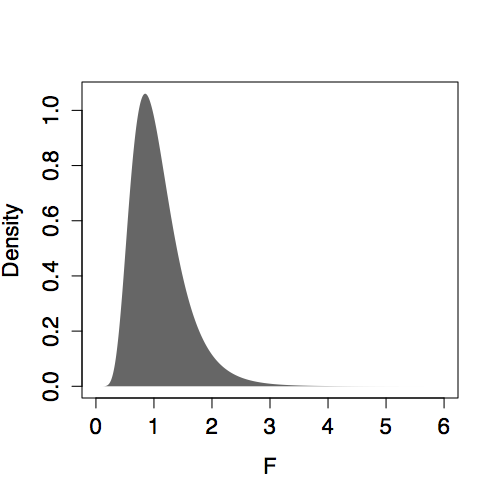
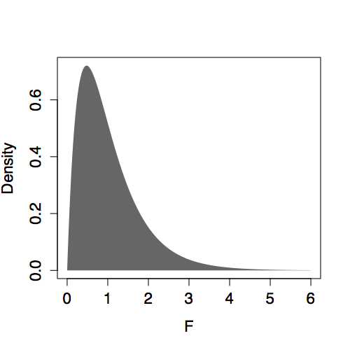
Aside: The shape of F

The shape of the F distribution depends on both n and m. Some of the distributions are shown for various m and n in Figure 14.6. Despite slight differences, the F distributions are all centered on 1. (In contrast, distributions of R² change shape substantially with m and n.) This steadiness in the F distribution makes it easy to interpret an F statistic by eye since a value near 1 is a plausible outcome from the null hypothesis. (The meaning of “near” reflects the width of the distribution: When n is much bigger than m, the the F distribution has mean 1 and standard deviation that is roughly √(2/m).)

Presenting F with m and n as the parameters violates a convention. The F distribution is always specified in terms of the degrees of freedom of the numerator m-1 and the degrees of freedom of the denominator n-m.

n=10, m=5	n=50, m=25
n=50, m=5	n=50, m=45

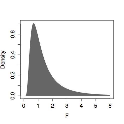Figure 14.6: F distribution for various n and m.

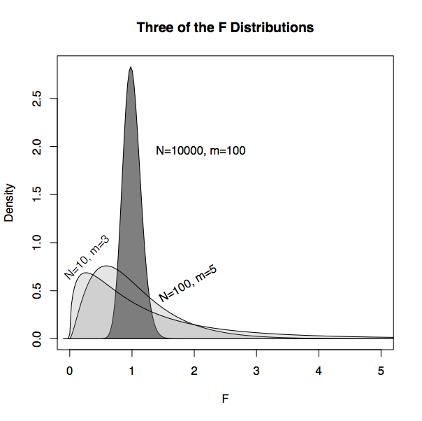
Figure 14.7: Three of the F distributions. When m and n-m are both large, the distribution is closely centered on F=1, the expected value for random model vectors.

Example: F and Astrology

Returning to the attempt to model age at marriage by astrological sign …

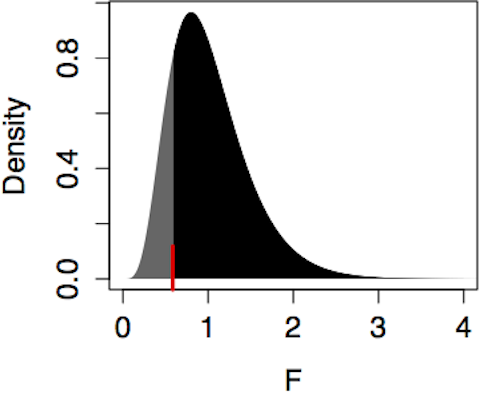
The model Age ~ Sign produced R² = 0.070 with m=12 model vectors and n=98 cases. The F statistic is therefore (0.070/11)/(0.930/86) = 0.585. Since F is somewhat less than 1, there is no reason to think that the Sign vectors are more effective than random vectors in explaining Age. Finding a p-value involves looking up the value F=0.585 in the F distribution with m-1=11 degrees of freedom in the numerator and n-m=86 degrees of freedom in the denominator. Figure 14.8 (left) shows this F distribution.

Age ~ Sign	Age ~ College
p < 0.836	p < 0.017

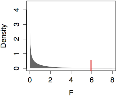
Figure 14.8: Finding a p-value from an F distribution always involves the area to the right of the test statistic, in this case marked by the ticks at F=0.585 (for Age ~ Sign) and F=5.93 (for Age ~ College).

The p-value is the probability of seeing an F value from this distribution that is larger than the observed value of F=0.585. From the figure, it’s easy to see that p is more than one-half since a majority of the distribution falls to the right of 0.585. Calculating it exactly using software gives p=0.836.

14.4 Interpreting the p-value

The p-value is a useful format for summarizing the strength of evidence that the data provide. But statistical evidence, like any other form of evidence, needs to be interpreted in context.

Multiple Comparisons

Keep in mind that a hypothesis test, particularly when p is near the conventional p<0.05 threshold for rejection of the null, is a very weak standard of evidence. Failure to reject the null may just mean that there isn’t enough data to reveal the patterns, or that important explanatory variables have not been included in the model.

But even when the p-value is below 0.05, it needs to be interpreted in the context within which the tested hypothesis was generated. Often, models are used to explore data, looking for relationships among variables. The hypothesis tests that stem from such an exploration can give misleadingly low p-values. To illustrate, consider an analogous situation in the world of crime. Suppose there were 20 different genetic markers evenly distributed through the population. A crime has been committed and solid evidence found on the scene shows that the perpetrator has a particular genetic marker, M, found in only 5% of the population. The police fan out through the city, testing passersby for the M marker. A man with M is quickly found and arrested.

Should he be convicted based on this evidence? Of course not. That this specific man should match the crime marker is unlikely, a probability of only 5%. But by testing large numbers of people who have no particular connection to the crime, it’s a guarantee that someone who matches will be found.

Now suppose that eyewitnesses had seen the crime at a distance. The police arrived at the scene and quickly cordoned off the area. A man, clearly nervous and disturbed, was caught trying to sneak through the cordon. Questioning by the police revealed that he didn’t live in the area. His story for why he was there did not hold up. A genetic test shows he has marker M. This provides much stronger, much more credible evidence. The physical datum of a match is just the same as in the previous scenario, but the context in which that datum is set is much more compelling.

The lesson here is that the p-value needs to be interpreted in context. The p-value itself doesn’t reveal that context. Instead, the story of the research project come into play. Have many different models been fitted to the data? If so, then it’s likely that one or more of them may have p < 0.05 even if the explanatory variables are not linked to the response.

It’s a grave misinterpretation of hypothesis testing to treat the p-value as the probability that the null hypothesis is true. Remember, the p-value is based on the assumption that the null hypothesis is true. A low p-value may call that assumption into doubt, but that doubt needs to be placed into the context of the overall situation.

Consider the unfortunate researcher who happens to work in a world where the null hypothesis is always true. In this world, each study that the researcher performs will produce a p-value that is effectively a random number equally likely to be anywhere between 0 and 1. If this researcher performs many studies, it’s highly likely that one or more of them will produce a p-value less than 0.05 even though the null is true.

Tempting though it may be to select a single study from the overall set based on its low p-value, it’s a mistake to claim that this isolated p-value accurately depicts the probability of the null hypothesis. Statistician David Freedman writes, “Given a significant finding … the chance of the null hypothesis being true is ill-defined – especially when publication is driven by the search for significance.” (Freedman 2008)

One approach to dealing with multiple tests is to adjust the threshold for rejection of the null to reflect the multiple possibilities that chance has to produce a small p-value. A simple and conservative method for adjusting for multiple tests is the Bonferroni correction. Suppose you perform k different tests. The Bonferroni correction adjusts the threshold for rejection downward by a factor of 1/k. For example, if you perform 15 hypothesis tests, rather than rejecting the null at a level of 0.05, your threshold for rejection should be 0.05/15 = 0.0033.

Another strategy is to treat multiple testing situations as “hypothesis generators.” Tests that produce low p-values are not to be automatically deemed as significant but as worthwhile candidates for further testing.(Saville 1990). Go out and collect a new sample, independent of the original one. Then use this sample to perform exactly one hypothesis test: re-testing the model whose low p-value originally prompted your interest. This common-sense procedure is called an out-of-sample test, since the test is performed on data outside the original sample used to form the hypothesis. In contrast, tests conducted on the data used to form the hypothesis are called in-sample tests. It’s appropriate to be skeptical of in-sample tests.

When reading work from others, it can be hard to know for sure whether a test is in-sample or out-of-sample. For this reason, researchers value prospective studies, where the data are collected after the hypothesis has been framed. Obviously, data from a prospective study must be out-of-sample. In contrast, in retrospective studies, where data that have already been collected are used to test the hypothesis, there is a possibility that the same data used to form the hypothesis are also being used to test it. Retrospective studies are often disparaged for this reason, although really the issue is whether the data are in-sample or out-of-sample. (Retrospective studies also have the disadvantage that the data being analyzed might not have been collected in a way that optimally addresses the hypothesis. For example, important covariates might have been neglected.)

Example: Multiple Jeopardy

You might be thinking: Who would conduct multiple tests, effectively shopping around for a low p-value? It happens all the time, even in situations where wrong conclusions have important implications.²

To illustrate, consider the procedures adopted by the US Government’s Office of Federal Contract Compliance Programs when auditing government contractors to see if they discriminate in their hiring practices. The OFCCP requires contractors to submit a report listing the number of applicants and the number of hires broken down by sex, by several racial/ethnic categories, and by job group. In one such report, there were 9 job groups (manager, professional, technical, sales workers, office/clerical, skilled crafts, operatives, laborers, service workers) and 6 discrimination categories (Black, Hispanic, Asian/Pacific Islander, American Indian/American Native, females, and people with disabilities).

According to the OFCCP operating procedures (Federal Contract Compliance Programs, n.d.), a separate hypothesis test with a rejection threshold of about 0.05 is to be undertaken for each job group and for each discrimination category, for example, discrimination against Black managers or against female sales workers. This corresponds to 54 different hypothesis tests. Rejection of the null in any one of these tests triggers punitive action by the OFCCP. Audits can occur annually, so there is even more potential for repeated testing.

Such procedures are not legitimately called hypothesis tests; they should be treated as screening tests meant to identify potential problem areas which can then be confirmed by collecting more data. A legitimate hypothesis test would require that the threshold be adjusted to reflect the number of tests conducted, or that a pattern identified by screening in one year has to be confirmed in the following year.

Significance vs Substance

It’s very common for people to misinterpret the p-value as a measure of the strength of a relationship, rather than as a measure for the evidence that the data provide. Even when a relationship is very slight, as indicated by model coefficients or an R², the evidence for it can be very strong so long as there are enough cases.

Suppose, for example, that you are studying how long patients survive after being diagnosed with a particular disease. The typical survival time is 10 years, with a standard deviation of 5 years. In your research, you have identified a genetic trait that explains some of the survival time: modeling survival by the genetics produces an R² of 0.01. Taking this genetic trait into account makes the survival time more predictable; it reduces the standard deviation of survival time from 5 years to 4.975 years. Big deal! The fact is, an R² of 0.01 does not reduce uncertainty very much; it leaves 99 percent of the variance unaccounted for.

To see how the F statistic stems from both R² = 0.01 and the sample size n, re-write the formula for F from Equation 14.1:

\(F = \frac{R²}{m-1} \Biggm/ \frac{1-R²}{n-m} \ \ \ \ \ \ \ \ \ \ \ \ \ \ \ \ \ \ \ \ \ (14.2)\)

\(\ \ \ \ = \left( \frac{n-m}{m-1} \right) \ \frac{R²}{1-R²}\)

$    = {}. $

The ratio R²/(1-R²) is a reasonable way to measure the substance of the result: how forceful the relationship is. The ratio (n-m)/(m-1) reflects the amount of data. Any relationship, even one that lacks practical substance, can be made to give a large F value so long as n is big enough. For example, taking m=2 in your genetic trait model, a small study with n=100 gives an F value of approximately 1: not significant. But if n=1000 cases were collected, the F value would become a hugely significant F=10. When used in a statistical sense to describe a relationship, the word “significant” does not mean important or substantial. It merely means that there is evidence that the relationship did not arise purely by accident from random variation in the sample.

Example: The Significance of Finger Lengths

The example in Section 14.4 commented on a study that found R² = 0.044 for the relationship between finger-length ratios and aggressiveness. The relationship was hyped in the news media as the “key to aggression.” (BBC News, 2005/03/04) The researchers who published the study(Bailey and Hurd 2005) didn’t characterize their results in this dramatic way. They reported merely that they found a statistically significant result, that is, p-value of 0.028. The small p-value stems not from a forceful correlation but from number of cases; their study, at n=134, was large enough to produce a value of F bigger than 4 even though the “substance”, R²/(1−R²), is only 0.046.

The researchers were careful in presenting their results and gave a detailed presentation of their study. They described their use of four different ways of measuring aggression: physical, hostility, verbal, and anger. These four scales were each used to model finger-length ratio for men and women separately. Here are the p-values they report:

Sex	Scale	R²	p-value
Males	Physical	0.044	0.028
	Hostility	0.016	0.198
	Verbal	0.008	0.347
	Anger	0.001	0.721
Females	Physical	0.010	0.308
	Hostility	0.001	0.670
	Verbal	0.001	0.778
	Anger	0.000	0.887

Notice that only one of the eight p-values is below the 0.05 threshold. The others seem randomly scattered on the interval 0 to 1, as would be expected if there were no relationship between the finger-length ratio and the aggressiveness scales. A Bonferroni correction to account for the eight tests gives a rejection threshold of 0.05/8 = 0.00625. None of the tests satisfies this threshold.

---

2. See Section 13.9 for another example.↩