Chapter 5 Confidence Intervals

It’s easy enough to calculate the mean or median within groups. Often the point of doing this is to support a claim that the groups are different, for instance that men are on average taller than women.

Less obvious to those starting out in statistics is the idea that a quantity such as the mean or median itself has limited precision. This isn’t a matter of the calculation itself. If the calculation has been done correctly, the resulting quantity is exactly right. Instead the limited precision arises from the sampling process that was used to collect the data. The exact mean or median relates to the particular sample you have collected. Had you collected a different sample, it’s likely that you would have gotten a somewhat different value for the quantities you calculate, the so-called sampling variability. One purpose of statistical inference is to characterize sampling variability, that is, to provide a quantitative meaning for “somewhat different value.”

5.1 The Sampling Distribution

An estimate of the limits to precision that stem from sampling variability can be made by simulating the sampling process itself. To illustrate, consider again the data in the TenMileRace table. These data give the running times of all 12,302 participants in a ten-mile long running race held in Washington, DC in March 2008.

Suppose want to describe how women’s running times differ from men’s. If you had to go out and collect your own data, you would likely take a random sample from the sampling frame. Suppose, for instance, that you collect a sample of size n = 200 runners and calculate the group-wise mean running time for men and women.

The results will be that men took, on average, about 88 minutes to run the 10 miles, while women took about 99 minutes. If you were to take another random sample of n = 200, you would get a somewhat different answer, perhaps 86 minutes for men and 98 for women. Each new random sample of n = 200 will generate a new result.

The sampling distribution describes how different the answers stemming from different random samples will be. The word “random” is very important here. Random sampling helps to ensure that the sample is representative of the population.

The process of generating the sampling distribution is shown in Figure 5.1. Take a random sample from the sampling frame and calculate the statistic of interest. (In this case, that’s the mean running time for men and for women.) Do this many times. Because of the random sampling process, you’ll get somewhat different results each time. The spread of those results indicates the limited precision that arises from sampling variability.

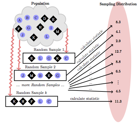
Figure 5.1: The sampling distribution reflects how the sample statistics would vary from one random sample to the next.

Historically, the sampling distribution was approximated using algebraic techniques. But it’s perfectly feasible to use the computer to repeat the process of random sampling many times and to generate the sampling distribution through a simulation.

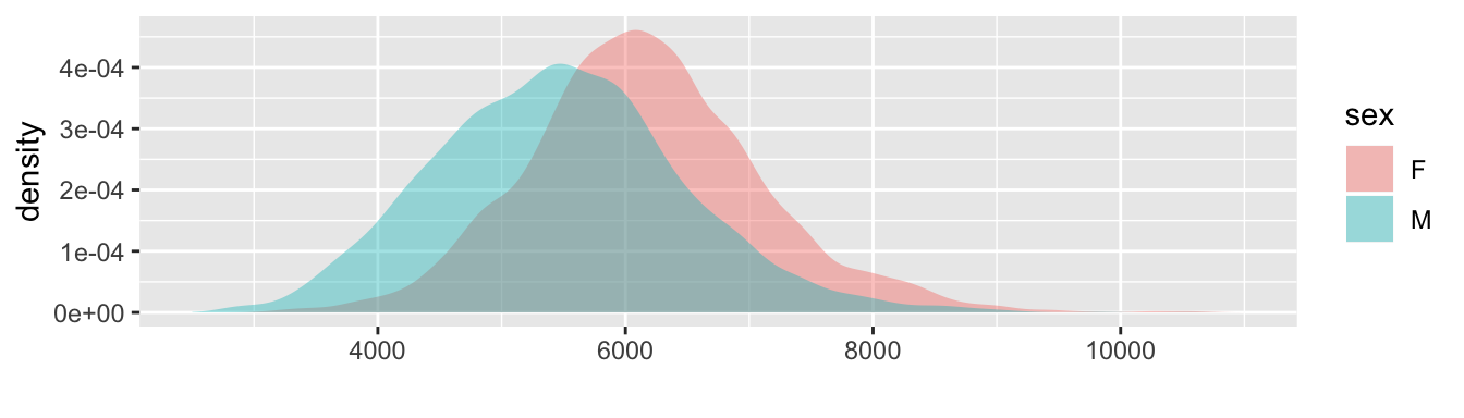
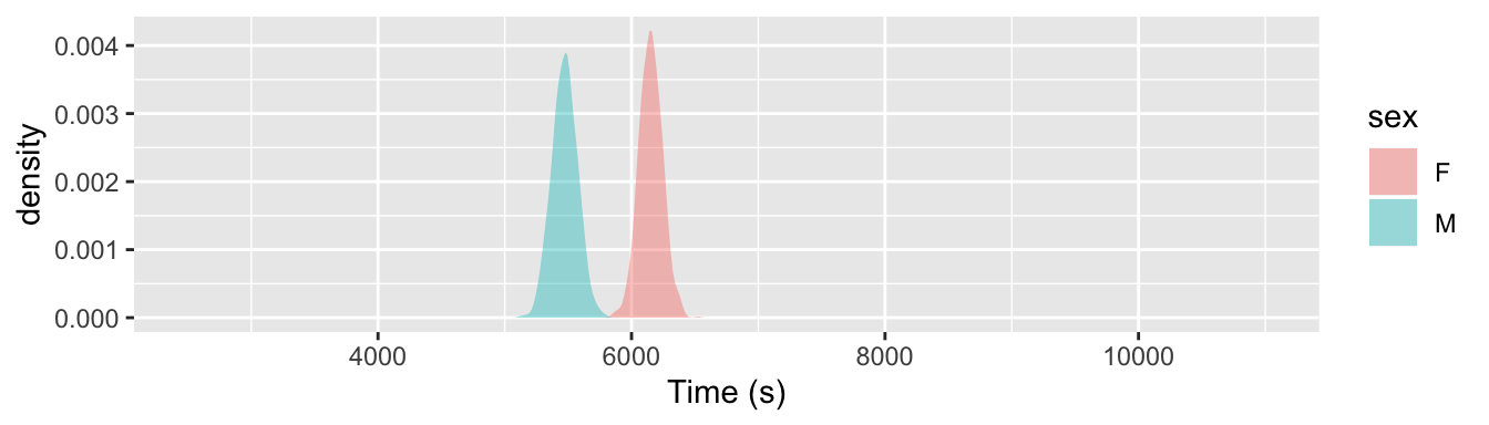
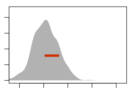
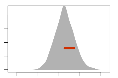
Figure 5.2: Comparing the distribution of the population of individuals (top) to the sampling distribution of the means of men’s and women’s running times for a sample of size n = 200 (bottom).

The sampling distribution depends on both the data and on the statistic being calculated. Figure 5.2 shows both the distribution of individual running times – the data themselves! – and the sampling distribution for the means of men’s and women’s running time for a sample of size n = 200.

Notice that the sampling distribution of the mean running times for n = 200 is much narrower than the individual data. That’s because, in taking the mean, the fast running times tend to cancel out the slow running times.

The usual way to quantify the precision of a measurement is called a confidence interval. This is commonly written in either of two equivalent ways:

• Plus-and-minus format 98.8 ± 1.7 minutes with 95% confidence
• Range format 97.1 to 100.5 minutes with 95% confidence.

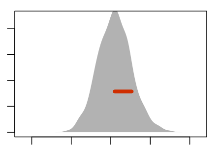
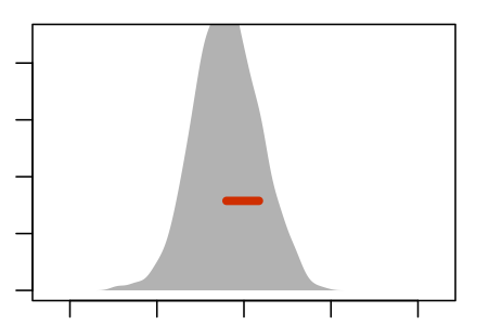
If the sample size had been smaller, the confidence interval would be bigger; that is, smaller samples result in less precise estimates. Figure 5.3 shows the sampling distribution for the mean of the running times for samples of size n = 50 and n = 800. Notice that when n=50, the sampling distribution is wide – the men’s mean and the women’s mean overlap somewhat. This is because n = 50 cases don’t allow a very precise statement to be made about the means. For instance, the 95% confidence interval for women is 98.8 ± 5.3 minutes and for men it’s 88.2 ± 5.8 minutes. In contrast, when n = 800, the sampling distribution is very narrow. All that data results in a very precise estimate: for women 98.8 ± 1.3 minutes and 88.2 ± 1.4 minutes for men.

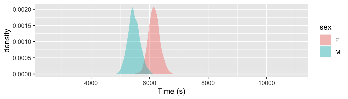
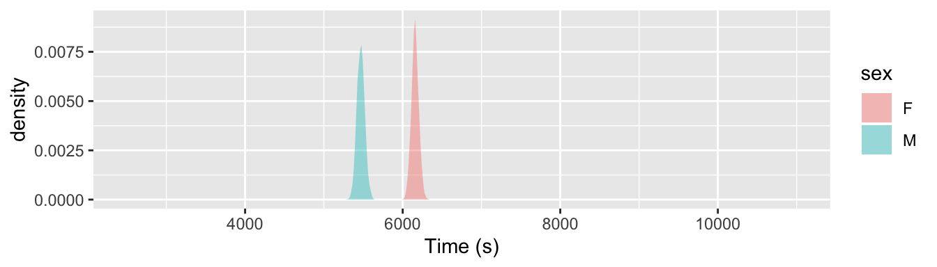
Figure 5.3: The sampling distributions of the mean of men’s and women’s running time for n = 50 and n = 800. A larger sample size gives a more precise estimate of the mean.

The logic of sampling distributions and confidence intervals applies to any statistic calculated from a sample, not just the means used in these examples but also proportions, medians, standard deviations, inter-quartile intervals, etc.

Aside: Precision and Sample Size

In keeping with the Pythagorean principle, it’s the square of the precision that behaves in a simple way, just as it’s the square of triangle edge lengths that add up in the Pythagorean relationship. As a rule, the square width of the sampling distribution scales with 1/n, that is, \[\mbox{width}^2 \propto \frac{1}{n}.\]

Taking square roots leads to the simple relationship of width with n: \[\mbox{width} \propto \frac{1}{\sqrt{n}}.\]

To improve your precision by a factor of two, you will need 4 times as much data. For ten times better precision, you’ll need 100 times as much data.

5.2 The Resampling Distribution & Bootstrapping

The construction of the sampling distribution by repeatedly collecting new samples from the population is theoretically sound but has a severe practical short-coming: It’s hard enough to collect a single sample of size n, but infeasible to repeat that work multiple times to sketch out the sampling distribution. And, if you were able to increase the number of cases in your sample, you would have included the new cases in your original sample: n would have been bigger to give you better precision. For almost all practical work, you need to estimate the properties of the sampling distribution from your single sample of size n.

One way to do this is called bootstrapping. The word itself is not very illuminating. It’s drawn from the phrase, “He pulled himself up by his own bootstraps,” said of someone who improves himself through his own efforts, without assistance.

To carry out a statistical bootstrap, you substitute your sample itself in place of the overall sampling frame, creating a hypothetical population that is easy to draw new samples from – Use the computer! – and can in many circumstances, be used to generate an approximation to the sampling distribution. The simple idea behind bootstrapping is to use the sample itself to stand for the population.

5.3 Re-sampling

The sample is already in hand, in the form of a data frame, so it’s easy to draw cases of it. Such new samples, taken from your original sample, not from the population, are called resamples : sampling from the sample.

Figure 5.4 illustrates how re-sampling works. There is just one sample drawn – with actual labor and expense – from the real population. Thereafter, the sample itself is used as a stand-in for the population and new samples are drawn from the sample.

Will such resamples capture the sampling variation that would be expected if you were genuinely drawing new samples from the population? An objection might come to mind: If you draw n cases out of a sample consisting of n cases, the resample will look exactly like the sample itself. No variability. This problem is easily overcome by sampling with replacement .

Whenever a case is drawn from the sample to put in a resample, the case is put back so that it is available to be used again. This is not something you would do when collecting the original sample; in sampling (as opposed to re-sampling) you don’t use a case more than once.

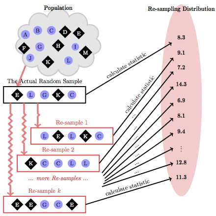
Figure 5.4: Re-sampling draws randomly from the sample to create new samples. Compare this process to the hypothetical sampling-distribution process in Figure 5.1.

The resamples in Figure 5.4 may seem a bit odd. They often repeat cases and omit cases. And, of course, any case in the population that was not included in the sample cannot be included in any of the resamples. Even so, the resamples do the job; they simulate the variation in model coefficients introduced by the process of random sampling.

The process of finding confidence intervals via re-sampling is called bootstrapping.

5.4 The Re-Sampling Distribution

It’s important to emphasize what the resamples do not and cannot do: they don’t construct the sampling distribution. The resamples merely show what the sampling distribution would look like if the population looked like your sample. The center of the re-sampling distribution from any given sample is generally not aligned exactly with the center of the population-based sampling distribution. However, in practice, the width of the re-sampling distribution is a good match to the width of the sampling distribution. The re-sampling distribution is adequate for the purpose of finding standard errors and margins of error.

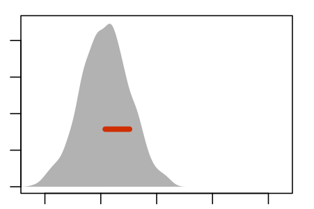
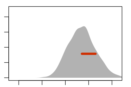
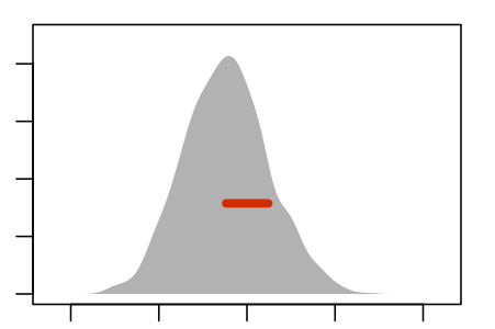
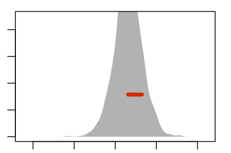
Figure 5.5 shows an experiment to demonstrate this. The panels show nine re-sampling distributions, each drawn from a single genuine sample of size n = 100 from the population. For each of the panels, that one genuine sample was the basis for drawing 1000 resamples. It’s the spread of the age coefficient across those 1000 resamples that’s displayed in the panel.

Some Resampling Distributions

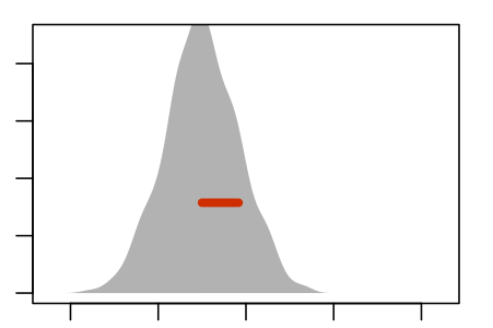Figure 5.5: Nine re-sampling distributions, each constructed from an individual sample from the population.

For comparison, here is the sampling distribution of the age coefficient in the running model. This was found by drawing 1000 genuine repeated samples of size n = 100 from the population.reflecting variation when sampling from the entire population rather than resampling from a single sample.

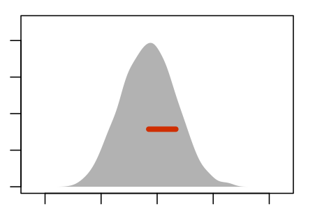
Figure 5.6: The sampling distribution

The re-sampling distribution varies across each panel, that is, across the nine different genuine samples used to generate the nine panels. Sometimes the resampling distribution is to the left of the sampling distribution, sometimes to the right, occasionally well aligned. Consistently, however, the re-sampling distributions have a standard error that is a close match to the standard error of the sampling distribution.

Example: The Precision of Grades

The “grade-point average” is widely used to describe a student’s academic performance. Grading systems differ from place to place. In the United States, it’s common to give letter grades with A the best grade, and descending through B, C, and D, and with E or F representing failure. You can’t average letters, so they are converted to numbers (i.e., A=4, B=3, and so on) and the numbers are averaged.

An individual typically sees his or her own grades in isolation, but institutions have large collections of information about those grades, including other information such as the instructor’s identity, the size of the class, etc. Here is of part of such an institutional database from a college with an enrollment of about 2000 students. This shows the information for a single student, ID 31509. Of course, the database contains information for many other students as well.

sessionID	grade	sid	grpt	dept	level	sem	enroll	iid
C1959	B+	S31509	3.33	Q	300	FA2001	13	i323
C2213	A-	S31509	3.66	i	100	SP2002	27	i209
C2308	A	S31509	4.00	O	300	SP2002	18	i293
C2344	C+	S31509	2.33	C	100	FA2001	28	i140
C2562	A-	S31509	3.66	Q	300	FA2002	22	i327
C2585	A	S31509	4.00	O	200	FA2002	19	i310
C2737	A	S31509	4.00	q	200	SP2003	11	i364
C2851	A	S31509	4.00	O	300	SP2003	14	i308
C2928	B+	S31509	3.33	O	300	FA2003	22	i316
C3036	B+	S31509	3.33	q	300	FA2003	21	i363
C3443	A	S31509	4.00	O	200	FA2004	17	i300

(The course name and other identifying information such as the department and instructor have been coded for confidentiality.) The student’s grade-point average is just the mean of the fourth column: 3.60.

What’s rarely or ever reported is the precision of this number. A simple 95% confidence interval on the mean of these 11 grades is 3.6± 0.3, that is, 3.3 to 3.9. It’s important to keep in mind that this confidence interval reflects the individual grades and the amount of grade data. A grade-point average of 3.6 does not by any means always come with a margin of error of ± 0.3 – the size of the margin of error depends on the line-by-line variability within the grade data and on the number of grades. More data gives more precise estimates.

5.5 The Confidence Level

In constructing a confidence interval, a choice is made about how to describe the sampling distribution (or, in practice, the re-sampling distribution). The conventional choice is a 95% coverage interval – the top and bottom limits that cover 95% of the distribution.

When constructing a confidence interval, the amount of coverage is called a confidence level and is often indicated with a phrase like “at 95% confidence.” The choice of 95% is conventional and uncontroversial, but sometimes people choose for good reasons or bad to use another level such as 99% or 90%.

Why not 100%? Because a 100% confidence interval would be too broad to be useful. In theory, 100% confidence intervals tend to look like -∞ to ∞. No information there! Complete confidence comes at the cost of complete ignorance.

The 95% confidence level is standard in contemporary science; it’s a convention. For that reason alone, it is a good idea to use 95% so that the people reading your work will tend to interpret things correctly.

The vocabulary of “confidence interval” and “confidence level” can be a little misleading. Confidence in everyday meaning is largely subjective, and you often hear of people being “over confident” or “lacking self-confidence.” It might be better if a term like “sampling precision interval” were used. In some fields, the term “error bar” is used informally, although “error” itself may have nothing to do with it; the precision stems from sampling variation.

5.6 Interpreting Confidence Intervals

Confidence intervals are easy to construct, whether by bootstrapping or other techniques. The are also very easy to misinterpret. One of the most common misinterpretations is to confuse the statement of the confidence interval with a statement about the individuals in the sample. For example, consider the confidence interval for the running times of men and women. Using the Cherry-Blossom data (with more than 12,000 runners), the 95% confidence interval for the mean of women’s times is 98.77 ± 0.35 minutes and for men it is 88.3 ± 0.36.

Do those confidence intervals suggest to you that men are consistently faster than women, for example that most men are faster than most women? There’s no justification for such a belief in the data themselves. Figure 5.2 (left) shows the distribution of running times broken down by sex; there is a lot of overlap.

Confidence intervals are often mistaken for being about individuals – the “typical” person, when a mean is involved – but they are really about the strength of evidence, about the precision of an estimate. There is a lot of evidence in the Cherry-Blossom data that the mean running times for men and women differ; with so much data, you can make a very precise statement about the means as shown by the narrow confidence interval. But the confidence interval does not tell you how much a typical individual differs from the mean.

Another tempting statement is, “If I repeated my study with a different random sample, the new result would be within the margin of error of the original result.” But that statement isn’t correct mathematically, unless your point estimate happens to align perfectly with the population parameter – and there’s no reason to think this is the case.

Treat the confidence interval just as an indication of the precision of the measurement. If you do a study that finds a statistic of 17 ± 6 and someone else does a study that gives 23 ± 5, then there is little reason to think that the two studies are inconsistent. On the other hand, if your study gives 17 ± 2 and the other study is 23 ± 1, then something seems to be going on; you have a genuine disagreement on your hands.

5.7 Confidence Intervals from Census Data

Recall the distinction between a sample and a census. A census involves every member of the population, whereas a sample is a subset of the population.

The logic of statistical inference applies to samples and is based on the variation introduced by the sampling process itself. Each possible sample is somewhat different from other possible samples. The techniques of inference provide a means to quantify “somewhat” and a standard format for communicating the imprecision that necessarily results from the sampling process.

But what if you are working with the population: a census not just a sample? For instance, the employment termination data is based on every employee at the firm, not a random sample.

One point of view is that statistical inference for a census is meaningless: the population is regarded as fixed and non random, so the population parameters are also fixed. It’s sampling from the population that introduces random variation.

A different view, perhaps more pragmatic, considers the population itself as a hypothetically random draw from some abstract set of possible populations. For instance, in the census data, the particular set of employees was influenced by a host of unknown random factors: someone had a particularly up or down day when being interviewed, an employee became disabled or had some other life-changing event.

Similarly, in the grade-point average data, you might choose to regard the set of courses taken by a student as fixed and non-random. If so, the idea of sampling precision doesn’t make sense. On the other hand, it’s reasonable to consider that course choice and grades are influenced by random factors: schedule conflicts, what your friend decided to take, which instructor was assigned, which particular questions were on the final exam, and so on.

You can certainly calculate the quantities of statistical inference from the complete population, using the internal, case-by-case variation as a stand-in for the hypothetical random factors that influenced each case in the population. Interpreting confidence intervals from populations in the same way as confidence intervals can provide a useful indication of the strength of evidence, and, indeed is recognized by courts when dealing with claims of employment discrimination. It does, however, rely on an untestable hypothesis about internal variation, which might not always be true.

Compare, for example, two possible extreme scenarios of course choice and grades. In one, students select courses on their own from a large set of possibilities. In the other scenario, every student takes exactly the same sequence of courses from the same instructors. In the first, it’s reasonable to calculate a confidence interval on the grade-point average and use this interval to compare the performance of two students. In the second scenario, since the students have all been in exactly the same situation, there might not be a good justification for constructing a confidence interval as if the data were from a random sample. For instance, there might be substantial internal variation because different instructors have different grading standards. But since every student had the same set of instructors, that variation shouldn’t be included in estimating sampling variation and confidence intervals.

The reality, for courses and grades at least, is usually somewhere between the two scenarios. The modeling techniques described in later chapters provide an approach to pulling apart the various sources of variation, rather than ascribing all of it to randomness and including all of it in the calculation of confidence intervals.