Chapter 8 Fitting Models to Data
With four parameters, I can fit an elephant; with five I can make it wiggle its trunk. – John von Neumann (1903-1957), mathematician and computer architect
The purpose of models is not to fit the data but to sharpen the questions. – Samuel Karlin (1924-2007), mathematician
The selection of variables and terms is part of the modeler’s art. It is a creative process informed by your goals, your understanding of how the system you are studying works, and the data you can collect. Later chapters will deal with how to evaluate the success of the models you create as well as general principles for designing effective models that capture the salient aspects of your system.
This chapter is about a technical matter: fitting, how to find the coefficients that best match the model you choose to the data you have collected.
Fitting a model – once you have specified the design – is an entirely automatic process that requires no human decision making. It’s ideally suited to computers and, in practice, you will always use the computer to find the best fit. Nevertheless, it’s important to understand the way in which the computer finds the coefficients. Much of the logic of interpreting models is based on how firmly the coefficients are tied to the data, to what extent the data dictate precise values of the coefficients. The fitting process reveals this. In addition, depending on your data and your model design, you may introduce ambiguities into your model that make the model less reliable than it could be. These ambiguities, which stem from redundancy and multicollinearity, are revealed by the fitting process.
8.1 The Least Squares Criterion
Fitting a model is somewhat like buying clothes. You choose the kind of clothing that you want: the cut, style, and color. There are usually several or many different items of this kind, and you have to pick the one that matches your body appropriately. In this analogy, the style of clothing is the model design – you choose this. Your body shape is like the data – you’re pretty much stuck with what you’ve got.
There is a system of sizes of clothing: the waist, hip, and bust sizes, inseam, sleeve length, neck circumference, foot length, etc. By analogy, these are the model coefficients. When you are in the fitting room of a store, you try on different items of clothing with a range of values of the coefficients. Perhaps you bring in pants with waist sizes 31 through 33 and leg sizes 29 and 30. For each of the pairs of pants that you try on, you get a sense of the overall fit, although this judgment can be subjective. By trying on all the possible sizes, you can find the item that gives the best overall match to your body shape.
Similarly, in fitting a model, the computer tries different values for the model coefficients. Unlike clothing, however, there is a very simple, entirely objective criterion for judging the overall fit called the least squares criterion. To illustrate, consider the following very simple data set of age and height in children:
age |
height |
|---|---|
| 5 | 80 |
| 7 | 100 |
| 10 | 110 |
| (years) | (cm) |
As the model design, take height ~ 1 + age. To highlight the link between the model formula and the data, here’s a way to write the model formula that includes not just the names of the variables, but the actual column of data for each variable. Each of these columns is called a vector. Note that the intercept vector is just a column of 1s.
height = c₁  + c₂
+ c₂ 
The goal of fitting the model is to find the best numerical values for the two coefficients c₁ and c₂.
To start, guess something, say, c₁ = 5 and c₂ = 10. Just a starting guess. Plugging in these guesses to the model formula gives a model value of height for each case.
height = 5 + 10 = 
Arithmetic with vectors is done in the ordinary way. Coefficients multiply each element of the vector, so that 10 gives  . To add or subtract two vectors means to add or subtract the corresponding elements:
  + gives
  .
.
The residuals tell you how the response values (that is, the actual heights) differ from the model value of height. For this model, the residuals are

The smaller the residuals, the better the model values match the actual response values.
The residual vector above is for the starting guess c₁ = 5 and c₂ = 10. Try another guess of the coefficients, say c₁ = 40 and c₂ = 8. Plugging in this new guess …
height = 
The residuals from the new coefficients are
Residuals given by … 
The central question of fitting is this: Which of the two model formulas is better?
Look at the first case – the first row of the data and therefore the first row of each vector. This first case is a five-year old who is 80 cm tall. Plugging in the value 80 cm to the model formula gives a model height of 55 cm from the starting-guess model. For the second-guess model, the model height is 80 cm – exactly right.
The residuals carry the information about how close the model values are to the actual value. For the first-guess model, the residual is −25 cm, whereas for the second-guess model the residual is zero. Obviously, the second-guess model is closer for this one case.
As it happens, the second-guess model is closer for the second case as well – the 7-year old who is 100 cm tall. The residual for this child is 23 cm for the starting-guess model and only 4 cm for the second-guess model. But for the third case – the 10-year old who is 110 cm tall – the residual from the first-guess model is better; it’s 5 cm, compared to a residual of −10 cm from the second-guess model.
It is not uncommon in comparing two formulas to find, as in this model, one formula is better for some cases and the other formula is better for other cases. This is not so different from clothing, where one item may be too snug in the waist but just right in the leg, and another item may be perfect in the waist but too long in the leg.
What’s needed is a way to judge the overall fit. In modeling, the overall fit of a model formula is measured by a single number: the sum of squares of the residuals. For the first formula, this is 25² + 23² + 5² = 1179. For the second formula, the sum of squares of the residuals is 0² + 4² + (−10)² = 116. By this measure, the second formula gives a much better fit.
To find the best fit, keep trying different formulas until one is found that gives the least sum of square residuals: in short, the least squares. The process isn’t nearly so laborious as it might seem. There are systematic ways to find the coefficients that give the least sum of square residuals, just as there are systematic ways to find clothing that fits without trying on every item in the store. The details of these systematic methods are not important here.
Using the least squares criterion, a computer will quickly find the
best coefficients for the
height vs age model to be c₁ = 54.211 $
and c₂ = = 5.789. Plugging in these coefficients to
the model formula produces fitted model values of
 , residuals of
 , and therefore a sum of square
residuals of 42.105, clearly much better than either previous two
model formulas.
, and therefore a sum of square
residuals of 42.105, clearly much better than either previous two
model formulas.
How do you know that the coefficients that the computer gives are indeed the best? You can try varying them in any way whatsoever. Whatever change you make, you will discover that the sum of square residuals is never going to be less than it was for the coefficients that the computer provided.
Because of the squaring, negative residuals contribute to the sum of square residuals in the same way as positive residuals; it’s the size and not the sign of the residual that matters when calculating whether a residual is big or small. Consequently, the smallest possible sum of square residuals is zero. This can occur only when the model formula gives the response values exactly, that is, when the fitted model values are an exact match with the response values. Because models typically do not capture all of the variation in the response variable, usually you do not see a sum of square residuals that is exactly zero. When you do get residuals that are all zeros, however, don’t start the celebration too early. This may be a signal that there is something wrong, that your model is too detailed.
It’s important to keep in mind that the coefficients found using the least squares criterion are the best possible but only in a fairly narrow sense. They are the best given the design of the model and given the data used for fitting. If the data change (for example, you collect new cases), or if you change the model design, the best coefficients will likely change as well. It makes sense to compare the sum of square residuals for two model formulas only when the two formulas have the same design and are fitted with the same data. So don’t try to use the sum of square residuals to decide which of two different designs are better. Tools to do that will be introduced in later chapters.
Aside: Why Square Residuals?
Why the sum of square residuals? Why not some other criterion? The answers are in part mathematical, in part statistical, and in part historical.
In the late 18th century, three different criteria were competing, each of which made sense:
- The least squares criterion, which seeks to minimize the sum of square residuals.
- The least absolute value criterion. That is, rather than the sum of square residuals, one looks at the sum of absolute values of the residuals.
- Make the absolute value of the residual as small as possible for the single worst case.
All of these criteria make sense in the following ways. Each tries to make the residuals small, that is, to make the fitted model values match closely to the response values. Each treats a positive residual in the same way as a negative residual; a mismatch is a mismatch regardless of whether the fitted values are too high or too low. The first and second criteria each combine all of the cases in determining the best fit.
The third criterion is hardly ever used because it allows one or two cases to dominate the fitting process – only the two most extreme residuals count in evaluating the model. Think of the third criterion as a dead end in the historical evolution of statistical practice.
Computationally, the least squares criterion leads to simpler procedures than the least absolute value criterion. In the 18th century, when computing was done by hand, this was a very important issue. It’s no longer so, and there can be good statistical reasons to favor a least absolute value criterion when it is thought that the data may contain outliers.
The least squares criterion is best justified when variables have a bell-shaped distribution. Insofar as this is the situation – and it often is – the least squares criterion is arguably better than least absolute value.
Another key advantage of the least squares criterion is in interpretation, as you’ll see in Section 8.8.
8.2 Partitioning Variation
A model is intended to explain the variation in the response variable using the variation in the explanatory variables. It’s helpful in quantifying the success of this to be able to measure how much variation there is in the response variable, how much has been explained, and how much remains unexplained. This is a partitioning of variation into parts.
Section 4.2 introduced the idea of partitioning variation in the context of simple group-wise models. There, it was shown that the variance – the square of the standard deviation – is a useful way to quantify variation because it has the property of exactly dividing total variation into parts: the variation of model values and the variation of the residuals.
The variance has this same useful partitioning property with least-squares models. Chapter 9 describes how the variance is used to construct a simple measure, called R², of the quality of fit of a model.
Aside: Partitioning and the Sum of Squares
Another partitioning statistic is the sum of squares. The sum of squares is deceptively simple. To find the sum of squares of the response variable, just square the value for each case and add them up. Similarly, you can find the sum of squares of the fitted model values and the sum of squares of the residuals. The partitioning property is that the sum of squares of the response variable exactly equals the sum of squares of the fitted model values plus the sum of squares of the residuals.
8.3 The Geometry of Least Squares Fitting
The fitting process involves vectors. Earlier, vectors were presented
as a column of numbers. Another way to regard vectors is as an
“arrow”: a direction and a length. For instance, the vector
 , when plotted in the usual Cartesian coordinate
plane, points to the north-northeast and has square-length 3² + 4²
= 5².
, when plotted in the usual Cartesian coordinate
plane, points to the north-northeast and has square-length 3² + 4²
= 5².
Consider a very simple model, A ~ B. Each of the vectors involved, A and B, has a length and a direction, something like this:
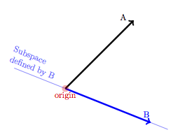
The process of least-squares fitting amounts to finding the point on the “subspace defined by B” that is as close as possible to A. You can do this by eye, if you like. Move your finger along the line that is the subspace defined by B to the point on that line that is as close as you can get to the tip of vector A. This is marked as the “Closest Pt.” in the figure below.
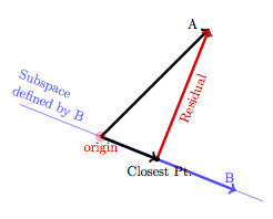
Of course, the closest point is not exactly the same as A. The vector that connects them is the residual vector.
Notice that choosing the fitted value as the closest point to A on the subspace defined by B means that the residual vector will be perpendicular to B. In statistics, the term that’s used for “perpendicular” is orthogonal.
One consequence of the orthogonality is that the three vectors involved – A, B, and the residual – form a right triangle. This is why the Pythagorean theorem applies and why it’s square quantities – the variance and the sum of squares – that have the partitioning property.
8.4 Redundancy
Data sets often contain variables that are closely related. For instance, consider the following data collected in 2009 on prices of used cars (the Ford Taurus model), the year the car was built, and the number of miles the car has been driven.
Price |
Year |
Mileage |
|---|---|---|
| 14997 | 2008 | 22613 |
| 8995 | 2007 | 53771 |
| 7990 | 2006 | 36050 |
| 18990 | 2008 | 25896 |
| … | … | … |
Although the year and mileage variables are different, they are related: older cars typically have higher mileage than newer cars. A group of students thought to see how price depends on year and mileage. After collecting a sample of 635 cars advertised on the Internet, they fit a model price ~ mileage + year. The coefficients came out to be:
price ~ mileage + year
| Term | Coefficient | Units |
|---|---|---|
| Intercept | −1136311.5 | dollars |
mileage |
−0.069 | dollars/mile |
year |
573.5 | dollars/year |
The coefficient on mileage is straightforward enough; according to the model the price of these cars typically decreases by 6.9 cents per mile. But the intercept seems strange: very big and negative. Of course this is because the intercept tells the model value at zero mileage in the year zero! They checked the plausibility of the model by plugging in values for a 2006 car with 50,000 miles: −1136312 − 0.069 × 50000 + 2006 × 573.50 giving
$10679.50 – a reasonable sounding price for such a car.
The students thought that the coefficients would make more sense if they were presented in terms of the age of the car rather than the model year. Since their data was from 2009, they calculated the age by taking 2009 − year. Then they fit the model price ~ mileage + age. Of course, there is no new information in the age variable that isn’t already in the year variable. Even so, the information is provided in a new way and so the coefficients in the new model are somewhat different.
price ~ mileage + age
| Term | Coefficient | Units |
|---|---|---|
| Intercept | 15850.0 | dollars |
mileage |
−0.069 | dollars/mile |
age |
−573.5 | dollars/year |
From the table, you can see that the mileage coefficient is unchanged, but now the intercept term looks much more like a real price: the price of a hypothetical brand new car with zero miles. The age coefficient makes sense; typically the cars decrease in price by $573.50 per year of age. Again, the students calculated the model for a 2006 car (thus age 3 years in 2009) with 50,000 miles: $10679.50, the same as before.
At first, the students were surprised by the differences between the two sets of coefficients. Then they realized that the two different model formulas give exactly the same model value for every car. This makes sense. The two models are based on exactly the same information. The only difference is that in one model the age is given by the model year of the car, in the other by the age itself.
The students decided to experiment. “What happens if we include both age and year in the model?” The started with the model price ~ mileage + year + age. They got these coefficients:
price ~ mileage + year + age
| Term | Coefficient | Units |
|---|---|---|
| Intercept | −1136311 | dollars |
mileage |
−0.069 | dollars/mile |
year |
573.5 | dollars/year |
age |
NA | dollars/year |
The model is effectively disregarding the age variable, reporting the coefficient as “NA”, not available.
The dual identity of age and year is redundancy. (The mathematical term is “linear dependence.”) It arises whenever an explanatory model vector can be modeled exactly in terms of the other explanatory vectors. Here, age can be computed by 2009 times the intercept plus \(−1\) times the year.
The problem with redundancy is that it creates ambiguity. Which of the four sets of coefficients in the table above is the right one? Whenever there is redundancy, there is more than one set of coefficients that gives the best fit of the model to the data.
In order to avoid this ambiguity, modeling software is written to spot any redundancy and drop the redundant model vectors from the model. One possibility would be to report a coefficient of zero for the redundant vector. But this could be misleading. For instance, the user might interpret the zero coefficient on Set 1 above as meaning that year isn’t associated with price. But that would be wrong; year is a very important determinant of price, it’s just that all the relationship is represented by the coefficient on age in Set 1. Rather than report a coefficient of zero, it’s helpful when software reports the redundancy by displaying a NA. This makes it clear that it is redundancy that is the issue and not that a coefficient is genuinely zero.
When model vectors are redundant, modeling software can spot the redundancy and do the right thing. But sometimes, the redundancy is only approximate, a situation called multi-collinearity. In such cases it’s important for you to be aware of the potential for problems; they will not be clearly marked by NA as happens with exact redundancy.
Example: Almost redundant
In collecting the Current Population Survey wage data, interviewers asked people their age and the number of years of education they had. From this, they computed the number of years of experience. They presumed that kids spend six years before starting school. So a 40-year old with 12 years of education would have 22 years of experience: 6 + 12 + 22 = 40. This creates redundancy of experience with age and education. Ordinarily, the computer could identify such a situation. However, there is a mistake in the CPS data. Case 350 is an 18-year old woman with 16 years of education. This seems hard to believe since very few people start their education at age 2. Presumably, either the age or education were mis-recorded. But either way, this small mistake in one case means that the redundancy among experience, age, and education is not exact. It also means that standard software doesn’t spot the problem when all three of these variables are included in a model. As a result, coefficients on these variables are highly unreliable.
With such multi-collinearity, as opposed to exact redundancy, there is a unique least-squares fit of the model to the data. However, this uniqueness is hardly a blessing. What breaks the tie to produce a unique best fitting set of coefficients are the small deviations from exact redundancy. These are often just a matter of random noise, arithmetic round-off, or mistakes as with case 350 in the Current Population Survey data. As a result, the choice of the winning set of coefficients is to some extent arbitrary and potentially misleading.
The costs of multi-collinearity can be measured when fitting a model. (See Section 12.6.) When the costs of multi-collinearity are too high, the modeler often chooses to take terms out of the model.
Aside: Redundancy – (Almost) Anything Goes
Even with the duplicate information in year and age, there is no mathematical reason why the computer could not have given coefficients for all four model terms in the model price ~ mileage + year + age. For example, any of the following sets of coefficients would give exactly the same model values for any inputs of year and mileage, with age being appropriately calculated from year.
| Term | Set 1 | Set 2 | Set 3 | Set 4 |
|---|---|---|---|---|
| Intercept | 15850.000 | −185050.000 | −734511.500 | −1136311.500 |
mileage |
−0.069 | −0.069 | −0.069 | 0.069 |
year |
0.000 | 100.000 | 373.500 | 573.500 |
age |
−573.500 | −473.500 | −200.000 | 0.000 |
The overall pattern is that the coefficient on age minus the coefficient on year has to be −573.5. This works because age and year are basically the same thing since age = 2009 − year.