Chapter 4 Groupwise Models
Seek simplicity and distrust it. – Alfred North Whitehead (1861-1947), mathematician and philosopher
This chapter introduces a simple form of statistical model based on separating the cases in your data into different groups. Such models are very widely used and will seem familiar to you, even obvious. They can be useful in very simple situations, but can be utterly misleading in others. Part of the objective of this chapter is to guide you to understand the serious limitations of such models and to critique the inappropriate, though all too common, use of group-wise models.
4.1 Grand and Group-wise Models
Consider these two statements:
Adults are about 67 inches tall.
Worldwide per-capita income in 2010 was about $16,000 per year.
Such statements lump everybody together into one group. But you can also divide things up into separate groups. For example:
Women are about 64 inches tall; men are about 69 inches tall.
Or consider this familiar-looking information about per-capita income:
| Country | Amount |
|---|---|
| Qatar | $127,660 |
| Bangladesh | $3891 |
| Luxembourg | $104,003 |
| Tajikistan | $3008 |
| Singapore | $87,855 |
| Zimbabwe | $1970 |
| United States | $57,436 |
| Afghanistan | $1919 |
| Switzerland | $59,561 |
| Haiti | $1784 |
| <!– http://en.w | ikipedia.org/wiki/List_of_countries_by_GDP_(PPP)_per_capita accessed on June 28, 2017 –> |
These sorts of statements, either in the grand mean form that puts everyone into the same group, or group-wise mean form where people are divided up into several groups, are very common.
People are used to this sort of division by sex or citizenship, so it’s easy to miss the point that these are only some of many possible variables that might be informative. Other variables that might also contribute to account for variation in people’s height are nutrition, parents’ height, ethnicity, etc.
It’s understandable to interpret such statements as giving “facts” or “data,” not as models. But they are representations of the situation which are useful for some purposes and not for others: in other words, models.
The group-wise income model, for instance, accounts for some of the person-to-person variation in income by dividing things up country by country. In contrast, the corresponding “grand” model is simply that per capita income worldwide is $16,000 – everybody in one group! The group-wise model is much more informative because there is so much spread: some people are greatly above the mean, some much, much lower, and a person’s country accounts for a lot of the variation.
The idea of averaging income by countries is just one way to display how income varies. There are many other ways that one might choose to account for variation in income. For example, income is related to skill level, to age, to education, to the political system in force, to the natural resources available, to health status, and to the population level and density, among many other things. Accounting for income with these other variables might provide different insights into the sources of income and to the association of income with other outcomes of interest, e.g., health. The table of country-by-country incomes is a statistical model in the sense that it attempts to explain or account for variation in income.
These examples have all involved situation where the cases are people, but in general you can divide up the cases in your data, whatever they be, into groups as you think best. The simplest division is really no division at all, putting every case into the same group. This might descriptively be called all-cases-the-same models, but you will usually hear them referred to by the statistic on which they are often based: the grand mean or the grand median. Here, “grand” is just a way of distinguishing them from group-wise quantities: grand versus group.
Given an interest in using models to account for variation, an all-cases-the-same model seems like a non-contender from the start – if everybody is the same, there is no variation. Even so, grand models are important in statistical modeling; they providing a starting point for measuring variation.
4.2 Accounting for Variation
Models explain or account for some (and sometimes all) of the case-to-case variation. If cases don’t vary one from the other, there is nothing to model!
It’s helpful to have a way to measure the “amount” of variation in a quantity so that you can describe how much of the overall variation a model accounts for. There are several such standard measures, described in Chapter 3:
- the standard deviation
- the variance (which is just the standard deviation squared)
- the inter-quartile interval
- the range (from minimum to maximum)
- coverage intervals, such as the 95% coverage intervals
Each of these ways of measuring variation has advantages and disadvantages. For instance, the inter-quartile interval is not much influenced by extreme values, whereas the range is completely set by them. So the inter-quartile interval has advantages if you are interested in describing a “typical” amount of variation, but disadvantages if you do not want to leave out even a single case, no matter how extreme or non-typical.
It turns out that the variance in particular has a property that is extremely advantageous for describing how much variation a model accounts for: the variance partitions the variation between that explained or accounted for by a model, and the remaining variation that remains unexplained or unaccounted for. This latter is called the residual variation.
To illustrate, consider the simple group-wise mean model, “Women are 64.1 inches tall, while men are 69.2 inches tall.” How does this model account for variation?
Measuring the person-to-person variation in height by the variance, gives a variation of 12.8 square-inches. That’s the total variation to be accounted for.
Now imagine creating a new data set that replaces each person’s actual height with what the model says. So all men would be listed at a height of 69.2 inches, and all women at a height of 64.1 inches. Those model values also have a variation, which can be measured by their variance: 6.5 square inches.
Now consider the residual, the difference between the actual height and the heights according to the model. A women who is 67 inches tall would have a residual of 2.9 inches – she’s taller by 2.9 inches than the model says. Each person has his or her own residual in a model. Since these vary from person to person, they also have a variance, which turns out to be 6.3 inches for this group-wise model of heights.
Notice the simple relationship among the three variances:
| Overall | Model | Residual | ||
|---|---|---|---|---|
| 12.8 | = | 6.5 | + | 6.3 |
This is the partitioning property of the variance: the overall case-by-case variation in a quantity is split between the variation in the model values and the variation in the residuals.
You might wonder why it’s the variance – the square of the standard deviation, with it’s funny units (square inches for height!) – that works for partitioning. What about the standard deviation itself or the IQR or other ways of describing variation? As it happens, the variance, uniquely, has the partitioning property. It’s possible to calculate any of the other measures of variation, but they won’t generally be such that the variation in the model values plus the variation in the residuals gives exactly the variation in the quantity being modeled. It’s this property that leads to the variance being an important measure, even though the standard deviation contains the same information and has more natural units.
The reason the variance is special can be explained in different ways, but for now it suffices to point out an analogous situation that you have seen before. Recall the Pythagorean theorem and the way it describes the relationship between the sides of a right triangle: if a and b are the lengths of the sides adjoining the right angle, and c is the length of the hypotenuse, then a² + b² = c². One way to interpret this is that sides a and b partition the hypotenuse, but only when you measure things in terms of square lengths rather than the length itself.
To be precise about the variance and partitioning … the variance has this property of partitioning for a certain kind of model – group-wise means and the generalization of that called linear, least-squares models that are the subject of later chapters – but those models are by far the most important. For other kinds of models, such as logistic models described in Chapter 16 there are other measures of variation that have the partitioning property.
Aside: The geometry of partitioning
The idea of partitioning is to divide the overall variation into parts: that accounted for by the model and that which remains: the residual.
This is done by assigning to each case a model value. The difference between the actual value and the model value is the residual. Naturally, this means that the model value plus the residual add up to the actual value. One way to think of this is in terms of a triangle: the model value is one side of the triangle, the residual is another side, and the actual values are the third side.
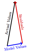
For reasons to be described in Chapter 8 it turns out that this triangle involves a right angle between the residuals and the model values. As such, the Pythagorean theorem applies and the square of the triangle side lengths add in the familiar way:
Model values² + Residuals² = Actual values² .
4.3 Group-wise Proportions
It’s often useful to consider proportions broken down, group by group. For example, In examining employment patterns for workers, it makes sense to consider mean or median wages in different groups, mean or median ages, and so on. But when the question has to do with employment termination – whether or not a person was fired – the appropriate quantity is the proportion of workers in each group who were terminated. For instance, in the job termination data, about 10% of employees were terminated. This differs from job level to job level, as seen in the table below. For instance, fewer than 2% of Principals (the people who run the company) were terminated. Staff were the most likely to be terminated.
| Administrative | Manager | Principal | Senior | Staff | |
|---|---|---|---|---|---|
| Retained | 92 | 92 | 98 | 90 | 88 |
| Terminated | 8 | 8 | 2 | 10 | 12 |
Figure 4.1 shows another way of looking at the termination data: breaking down the groups according to age and, within each group, showing the fraction of workers who were terminated. The graph suggests that workers in their late 60’s were substantially more likely to be fired. This might be evidence for age discrimination, but there might be other reasons for the pattern. For instance, it could be that those employees in their 60s were people who failed to be promoted in the past, or who were making relatively high salaries, or who were planning to retire soon. A more sophisticated model would be needed to take such factors into account.
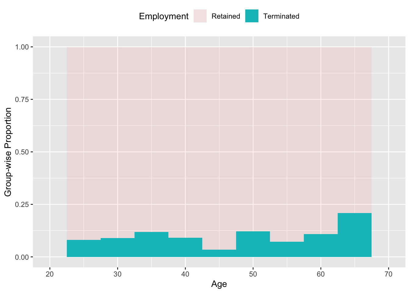
Figure 4.1: The proportion of workers who were terminated broken into groups according to age.
4.4 What’s the Precision?
The main point of constructing group-wise models is to be able to support a claim that the groups are different, or perhaps to refute such a claim. In thinking about differences, it’s helpful to distinguish between two sorts of criteria:
- Whether the difference is substantial or important in terms of the phenomenon that you are studying. For example, Administrative workers in the previous example were terminated at a rate of 8.27%, whereas Managers were terminated at a rate of 8.16%. This hardly makes a difference.
- How much evidence there is for any difference at all. This is a more subtle point.
In most settings, you will be working with samples from a population rather than the population itself. In considering a group difference, you need to take into account the random nature of the sampling process, which leads to some randomness is the group-wise statistics. If different cases had been included in the sample, the results would be different.
Quantifying and interpreting this sampling variability is an important component of statistical reasoning. The techniques to do so are introduced in Chapter 5 and then expanded in later chapters. But before moving on to the techniques for quantifying sampling variability, consider the common format for presenting it: the confidence interval.
A confidence interval is a way of expressing the precision or repeatability of a statistic, how much variation would likely be present across the possible different random samples from the population. In format, it is a form of coverage interval, typically taken at the 95% level, and looks like this:
68.6 ± 3.3
The first number, 68.6 here, is called the point estimate, and is the statistic itself. The second number, the margin of error, reflects how precise the point estimate is. There is a third number, sometimes stated explicitly, sometimes left implicit, the confidence level, which is the level of the coverage interval, typically 95%.
Like other coverage intervals, a confidence interval leaves out the extremes. You can think of this as arranging the confidence interval to reflect what plausibly might happen, rather than the full extent of the possibilities, no matter how extreme or unlikely.
4.5 Misleading Group-wise Models
Group-wise models appear very widely, and are generally simple to explain to others and to calculate, but this does not mean they serve the purposes for which they are intended. To illustrate, consider a study done in the early 1970s in Whickham, UK, that examined the health consequences of smoking. (Appleton, French, and MPJ 1996) The method of the study was simple: interview women to find out who smokes and who doesn’t. Then, 20 years later, follow-up to find out who is still living.
Examining the data Whickham shows that, after 20 years, 945 women in the study were still alive out of 1315 total: a proportion of 72% . Breaking this proportion into group-wise into smokers and non-smokers gives
- Non-smokers: 68.6% were still alive.
- Smokers: 76.1% were still alive.
Before drawing any conclusions, you should know what is the precision of those estimates. Using techniques to be introduced in the next chapter, you can calculate a 95% confidence interval on each proportion:
- Non-smokers: 68.6 ± 3.3% were still alive.
- Smokers: 76.1 ± 3.7% were still alive.
The 95% confidence interval on the difference in proportions is 7.5 ± 5.0 percentage points. That is, the data say that smokers were more likely than non-smokers to have stayed alive through the 20-year follow up period.
Perhaps you are surprised by this. You should be. Smoking is convincingly established to increase the risk of dying (as well as causing other health problems such as emphysema).
The problem isn’t with the data. The problem is with the group-wise approach to modeling. Comparing the smokers and non-smokers in terms of mortality doesn’t take into account the other differences between those groups. For instance, at the time the study was done, many of the older women involved had grown up at a time when smoking was uncommon among women. In contrast, the younger women were more likely to smoke. You can see this in the different ages of the two groups:
- Among non-smokers the average age is 48.7 ± 1.3.
- Among smokers the average age is 44.7 ± 1.4.
You might think that the difference of four years in average ages is too small to matter. But it does, and you can see the difference when you use modeling techniques to incorporate both age and smoking status as explaining mortality.
Since age is related to smoking, the question the group-wise model asks is, effectively, “Are younger smokers different in survival than older non-smokers?” This is probably not the question you want to ask. Instead, a meaningful question would be, “Holding other factors constant, are smokers different in survival than non-smokers?”
You will often see news reports or political claims that attempt to account for or dismiss differences by appealing to “other factors.” This is a valuable form of argument, but it ought to be supported by quantitative evidence, not just an intuitive sense of “small” or “big.” The modeling techniques introduced in the following chapters enable you to do consider multiple factors in a quantitative way.
A relatively simple modeling method called stratification can illustrate how this is possible.
Rather than simply dividing the Whickham data into groups of smokers and non-smokers, divide it as well into groups by age. Table 4.3 shows survival percentages done this way:
| smoker | [18,30) | [30,40) | [40,54) | [54,64) | [64,80) |
|---|---|---|---|---|---|
| No | 0.980 | 0.957 | 0.886 | 0.664 | 0.225 |
| Yes | 0.973 | 0.960 | 0.797 | 0.570 | 0.255 |
Within each age group, smokers are less likely than non-smokers to have been alive at the 20-year follow-up, especially in the older groups. By comparing people of similar ages – stratifying or disaggregating the data by age – the model is effectively “holding age constant.”
You may rightly wonder whether the specific choice of age groups plays a role in the results. You also might wonder whether it’s possible to extend the approach to more than one stratifying variable, for instance, not just smoking status but overall health status. The following chapters will introduce modeling techniques that let you avoid having to divide variables like age into discrete groups and that allow you to include multiple stratifying variables.