Chapter 18 Experiment
The true method of knowledge is experiment. – William Blake (1757-1827), English poet, painter, and print-maker
A theory is something nobody believes, except the person who made it. An experiment is something everybody believes, except the person who made it. – Albert Einstein (1879-1955), physicist
18.1 Experiments
The word “experiment” is used in everyday speech to mean a course of action tentatively adopted without being sure of the eventual outcome. (“New Oxford American Dictionary” 2015) You can experiment with a new cookie recipe; experiment by trying a new bus route for getting to work; experiment by planting some new flowers to see how they look.
Experimentation is at the core of the scientific method. Albert Einstein said, “[The] development of Western Science is based on two great achievements – the invention of the formal logical system (in Euclidean geometry) by the Greek philosophers, and the discovery of the possibility to find out causal relationships by systematic experiment (during the Renaissance).” (Boorstin 1995)
Scientific experimentation is, as Einstein said, systematic. In the everyday sense of experimentation, to try out a new cookie recipe, you cook up a batch and try them out. You might think that the experiment becomes scientific when you measure the ingredients carefully, set the oven temperature and timing precisely, and record all your steps in detail. Those are certainly good things to do, but a crucial aspect of systematic experimentation is comparison .
Two distinct forms of comparison are important in an experiment. One form of comparison is highlighted by the phrase “controlled experiment.” " A controlled experiment involves a comparison between two interventions: the one you are interested in trying out and another one, called a control, that provides a baseline or basis for comparison. In the cookie experiment, for instance, you would compare two different recipes: your usual recipe (the control) and the new recipe (called the treatment). Why? So that you can put the results for the new recipe in an appropriate context. Perhaps the reason you wanted to try a new recipe is that you were particularly hungry. If so, it’s likely that you will like the new recipe even if were not so good as your usual one. By comparing the two recipes side by side, a controlled experiment helps to reduce the effects of factors such as your state of hunger. (The word “controlled” also suggests carefully maintained experimental conditions: measurements, ingredients, temperature, etc. While such care is important in successful experiments, the phrase “controlled experiment” is really about the comparison of two or more different interventions.)
Another form of comparison in an experiment concerns intrinsic variability. The different interventions you compare in a controlled experiment may be affected by factors other than your intervention. When these factors are unknown, they appear as random variation. In order to know if there is a difference between your interventions – between the treatment and the control – you have to do more than just compare treatment and control. You have to compare the observed treatment-vs-control difference to that which would be expected to occur at random. The technical means of carrying out such a comparison is, for instance, the F statistic in ANOVA. When you carry out an experiment, it’s important to establish the conditions that will enable such a comparison to be carried out.
A crucial aspect of experimentation involves causation. An experiment does not necessarily eliminate the need to consider the structure of a hypothetical causal network when selecting covariates. However, the experiment actually changes the structure of the network and in so doing can radically simplify the system. As a result, experiments can be much easier to interpret, and much less subject to controversy in interpretation than an observational study.
18.2 Experimental Variables and Experimental Units
In an experiment, you, the experimenter, intervene in the system.
- You choose the experimental units , the material or people or animals to which the control and treatment will be applied. When the “unit” is a person, a more polite term is experiment subject .
- You set the value of one or more variables – the experimental variables – for each experimental unit.
The experimenter then observes or measures the value of one or more variables for each experimental unit: a response variable and perhaps some covariates.
The choice of the experimental variables should be based on your understanding of the system under study and the questions that you want to answer. Often, the choice is straightforward and obvious; sometimes it’s clever and ingenious. For example, suppose you want to study the possibility that the habit of regularly taking a tablet of aspirin can reduce the probability of death from stroke or heart attack in older people. The experimental variable will be whether or not a person takes aspirin daily. In addition to setting that variable, you will want to measure the response variable – the person’s outcome, e.g., the age of their eventual death – and covariates such as the person’s age, sex, medical condition at the onset of the study, and so on.
Or, suppose you want to study the claim that keeping a night-light on during sleeping hours increases the chances that the child will eventually need glasses for near-sightedness. The experimental variable is whether or not the child’s night light is on, or perhaps how often it is left on. Other variables you will want to measure are the response – whether the child ends up needing glasses – and the relevant covariates: the child’s age, sex, whether the parents are nearsighted, and so on.
In setting the experimental variable, the key thing is to create variability, to establish a contrast between two or more conditions. So, in the aspirin experiment, you would want to set things up so that some people regularly take aspirin and others do not. In the nearsightedness experiment, some children should be set to sleep in bedrooms with nightlights on and others in bedrooms with nightlights off.
Sometimes there will be more than one variable that you want to set experimentally. For instance, you might be interested in the effects of both vitamin supplements and exercise on health outcomes. Many people think that an experiment involves setting only one experimental variable and that you should do a separate experiment for each variable. There might be situations where this is sensible, but there can be big advantages in setting multiple experimental variables in the same experiment. (Later sections will discuss how to do this effectively – for instance it can be important to arrange things so that the experimental variables are mutually orthogonal.) One of the advantages of setting experimental variables simultaneously has to do with the amount of data needed to draw informative conclusions. Another advantage comes in the ability to study interactions between experimental variables. For example, it might be that exercise has different effects on health depending on a person’s nutritional state.
The choice of experimental units depends on many factors: practicality, availability, and relevance. For instance, it’s not so easy to do nutritional experiments on humans; it’s hard to get them to stick to a diet and it often takes a long time to see the results. For this reason, many nutritional experiments are done on short-living lab animals. Ethical concerns are paramount in experiments involving potentially harmful substances or procedures.
Often, it’s sensible to choose experimental units from a population where the effect of your intervention is likely to be particularly pronounced or easy to measure. So, for example, the aspirin experiment might be conducted in people at high risk of stroke or heart attack.
On the other hand, you need to keep in mind the relevance of your experiment. Studying people at the very highest risk of stroke or heart attack might not give useful information about people at a normal level of risk.
Some people assume that the experimental units should be chosen to be as homogeneous as possible; so that covariates are held constant. For example, the aspirin experiment might involve only women aged 70. Such homogeneity is not necessarily a good idea, because it can limit the relevance of the experiment. It can also be impractical because there may be a large number of covariates and there might not be enough experimental units available to hold all of them approximately constant.
One argument for imposing homogeneity is that it simplifies the analysis of the data collected in the experiment. This is a weak argument; analysis of data is typically a very small amount of the work and you have the techniques that you need to adjust for covariates. In any event, even when you attempt to hold the covariates constant by your selection of experimental units, you will often find that you have not been completely successful and you’ll end up having to adjust for the covariates anyway. It can be helpful, however, to avoid experimental units that are outliers. These outlying units can have a disproportionate influence on the experimental results and increase the effects of randomness.
A good reason to impose homogeneity is to avoid accidental correlations between the covariates and the experimental variables. When such correlations exist, attempts to untangle the influence of the covariates and experimental variables can be ambiguous, as described in Section 15.3. For instance, if all the subjects who take aspirin are women, and all the subjects who don’t take aspirin are men, how can you decide whether the result is due to aspirin or to the person’s sex?
There are other ways than imposing homogeneity, however, to avoid correlations between the experimental variables and the covariates. Obviously, in the aspirin experiment, it makes sense to mix up the men and women in assigning them to treatment or control. More formally, the general idea is to make the experimental variables orthogonal to covariates – even those covariates that you can’t measure or that you haven’t thought to measure. Section 18.6 shows some ways to do this.
Avoiding a confounding association between the experimental variables and the covariates sometimes has to be done through the experimental protocol. A placebo, from the Latin “I will please,” is defined as “a harmless pill, medicine, or procedure prescribed more for the psychological benefit to the patient than for any physiological effect.” (“New Oxford American Dictionary” 2015) In medical studies, placebos are used to avoid the confounding effects of the patient’s attitude toward their condition.
If some subjects get aspirin and others get nothing, they may behave in different ways. Think of this in terms of covariates: Did the subject take a pill (even if it didn’t contain aspirin)? Did the subject believe he or she was getting treated? Perhaps the subjects who don’t get aspirin are more likely to drink alcohol, upset at having been told not to take aspirin and having heard that a small amount of daily alcohol consumption is protective against heart attacks. Perhaps the patients told to take aspirin tend not to take their vitamin pills: “It’s just too much to deal with.”
Rather than having your control consist of no treatment at all, use a placebo in order to avoid such confounding. Of course, it’s usually important that the subjects be unaware whether they have been assigned to the placebo group or to the treatment group. An experiment in which the subjects are in this state of ignorance is called a blind experiment.
There is evidence that for some conditions, particularly those involving pain or phobias, placebos can have a positive effect compared to no treatment. (Hrobjartsson and Gotzcsche 2004,wampold-2005) This is the placebo effect. Many doctors also give placebos to avoid confrontation with patients who demand treatment. (Hrobjartsson and Norup 2003) This often takes the form of prescribing antibiotics for viral infections.
It can also be important to avoid accidental correlations created by the researchers between the experimental variables and the covariates. It’s common in medical experiments to keep a subject’s physicians and nurses ignorant about whether the subject is in the treatment or the control group. This prevents the subject from being treated differently depending on the group they are in. Such experiments are called double blind. (Of course, someone has to keep track of whether the subject received the treatment or the placebo. This is typically a statistician who is analyzing the data from the study but is not involved in direct contact with the experimental subjects.)
In many areas, the measured outcome is not entirely clear and can be influenced by the observer’s opinions and beliefs. In testing the Salk polio vaccine in 1952, the experimental variable was whether the child subject got the vaccine or not. (See the account in (Freedman, Purves, and Pisani 2007).) It was important to make the experiment double-blind and painful measures were taken to make it so; hundreds of thousands of children were given placebo shots of saline solution. Why? Because in many cases the diagnosis of mild polio is ambiguous; it might be just flu. The diagnostician might be inclined to favor a diagnosis of polio if they thought the subject didn’t get the vaccine. Or perhaps the opposite, with the physician thinking to himself, “I always thought that this new vaccine was dangerous. Now look what’s happened.”
Example: Virtues of Doing Surgery while Blind
In order to capture the benefits of the placebo effect and, perhaps more important, allow studies of the effectiveness of surgery to be done in a blind or double-blind manner, sham surgery can be done. For example, in a study of the effectiveness of surgery for osteoarthritis of the knee, some patients got actual arthroscopic surgery while the placebo group had a simulated procedure that included actual skin incisions.(Moseley and al. 2002) Sham brain surgery has even been used in studying a potential treatment for Parkinson’s disease.(Freeman 1999) Needless to say, sham surgery challenges the notion that a placebo is harmless. A deep ethical question arises: Is the harm to the individual patient sufficiently offset by the gains in knowledge and the corresponding improvements in surgery for future patients?
Example: Oops! An accidental correlation!
You are a surgeon who wants to test out a new and difficult operation to cure a dangerous condition. Many of the subjects in this condition are in very poor health and have a strong risk of not surviving the surgery, no matter how effective the surgery is at resolving the condition. So you decide, sensibly, to perform the operation on those who are in good enough health to survive and use as controls those who aren’t in a position to go through the surgery. You’ve just created a correlation between the experimental variable (surgery or not) and a covariate (health).
18.3 Choosing levels for the experimental variables
In carrying out an experiment, you set the experimental variables for each experimental unit. When designing your experiment, you have to decide what levels to impose on those variables. That’s the subject of this section. A later section will deal with how to assign the various levels among the experimental units.
Keep in mind these two principles:
- Comparison. The point of doing a systematic experiment is to contrast two or more things. Another way of thinking about this is that in setting your experimental variable, you create variability. In analyzing the data from your experiment you will use this variability in the experimental variables.
- Relevance. Do the levels provide a contrast that guides meaningful conclusions. Is the difference strong enough to cause an observable difference in outcomes?
It’s often appropriate to set the experimental variable to have a “control” level and a “treatment” level. For instance, placebo vs aspirin, or night-light off vs night-light on. When you have two such levels, a model “response ~ experimental variable” will give one coefficient that will be the difference between the treatment and the control and another coefficient – the intercept – that is the baseline.
Make sure that the control level is worthwhile so that the difference between the treatment and control is informative for the question you want to answer. Try to think what is the interesting aspect of the treatment and arrange a control that highlights that difference. For example, in studying psychotherapy it would be helpful to compare the psychotherapy treatment to something that is superficially the same but lacking the hypothesized special feature of psychotherapy. A comparison of the therapy with a control that involves no contact with the subject whatsoever may really be an experiment about the value of human contact itself rather than the value of psychotherapy.
Sometimes it’s appropriate to arrange more than two levels of the experimental variables, for instance more than one type of treatment. This can help tease apart effects from different mechanisms. It also serves the pragmatic purpose of checking that nothing has gone wrong with the overall set-up. For instance, a medical experiment might involve a placebo, a new treatment, and an established treatment. In experiments in biology and chemistry, where the measurement involves complicated procedures where something can go wrong (for instance, contamination of the material being studied) it’s common to have three levels of the experimental variable: a treatment, a positive control, and a negative control that gives a clear signal if something is wrong in the procedure or materials.
Often, the experimental variable is naturally quantitative: something that can be adjusted in magnitude. For instance, in an aspirin experiment, the control would be a daily dose of 0mg (delivered via placebo pill) and the treatment might be a standard dose of 325 mg per day. Should you also arrange to have treatments that are other levels, say 100 mg per day or 500 mg per day? It’s tempting to do so. But for the purposes of creating maximal variability in the experimental variable, it’s best to set the treatment and control at opposite ends of whatever the relevant range is: say 0 and 325 mg per day.
It can be worthwhile, however, to study the dose-response relationship. For example, it appears that a low dose of aspirin (about 80 mg per day) is just as effective as higher dosages in preventing cardiovascular disease.(Campbell et al. 2007) Put yourself in the position of a researcher who wants to test this hypothesis. You start with some background literature – previous studies have established that a dose of 325 mg per day is effective. You want to test a dose of one-quarter of that: 80 mg per day. It’s helpful if your experimental variable involves at least three levels: 0 mg (the control, packaged in a placebo), 80 mg, and 325 mg. Why not just use two levels, say 0 and 80 mg, or perhaps 80 and 325 mg? So that you can demonstrate that your overall experimental set up is comparable to that of the background literature and so that you can, in your own experiment, compare the responses to 80 and 325 mg.
When you analyze the data from such a multi-level experimental variable, make sure to include nonlinear transformation terms in your model. The model “response ~ dose” will not be able to show that 80 mg is just as effective as 325 mg; the linear form of the model is based on the assumption that 80 mg will be only about one-quarter as effective as 325 mg. If your interest is to show that 80 can be just as effective as 325 mg, you must include additional terms, for instance response ~ (dose > 0) + (dose > 80)
18.4 Replication
Perhaps it seems obvious that you should include multiple experimental units: replication. For example, in studying aspirin, you want to include many subjects, not just a single subject at the control level and a single subject at the treatment level.
But how many? To answer this question, you need to understand the purposes of replication. There are at least two:
- Be able to compare the variability associated with the experimental variables from the background variability that arises from random sampling. This is done, for instance, when looking at statistical significance using an F statistic. (See Section 14.2.)
- Increase the ability of your experiment to detect a difference if it really does exist: the power of your experiment.
In setting the number of cases in your experiment, you need first to ensure that you have some non-zero degree of freedom in your residual. If not, you won’t be able to compute an F value at all, or, more generally, you won’t be able to compare the variability associated with your experimental variables with the variability described as random.
Second, you should arrange things so that the p-value that you would expect, assuming that the experimental variable acts as you anticipate, is small enough to give you a significant result. This relates to the issue of the power of your experiment: the probability that you would get a significant result in a world where the experimental variable acts as you anticipate. The relationship between sample size and power is described in Section 13.7.
18.5 Experiments vs Observations
Why do an experiment when you can just observe the “natural” relationships? For example, rather than dictating to people how much aspirin they take, why not just measure the amount they take on their own, along with appropriate covariates, and then use modeling to find the relationships?
To illustrate, Figure 18.1 shows a hypothetical causal network that models the relationship between aspirin intake and stroke:
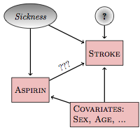
Figure 18.1: A hypothetical causal network for the relationship between aspirin and stroke.
Included in this network is a latent (unmeasured, and perhaps unmeasurable) variable: sickness. The link between sickness and aspirin is intended to account for the possibility that sicker subjects – those who believe themselves to be at a higher risk of stroke – might have heard of the hypothesized relationship between aspirin and risk of stroke and are medicating themselves at a higher rate than those who don’t believe themselves to be sick.
There are three pathways between aspirin and stroke. The direct pathway, marked ???, is of principal interest. One backdoor pathway goes through the sickness latent variable: aspirin⥢ sickness⥤ stroke. Another backdoor pathway goes through the covariates: aspirin⥢ covariates⥤ stroke.
If you want to study the direct link between aspirin and stoke, you need to block the backdoor pathways. If you don’t, you can get misleading results. For instance, the increased risk of stroke indicated by the sickness variable might make it look as if aspirin consumption itself increases the risk of stroke, even if the direct effect of aspirin is to decrease the risk. Both the backdoor pathways are correlating pathways. To block them, you need to include sickness and the covariates (sex, age, etc.) in your model, e.g., a model like this:
stroke ~ aspirin + sickness + age + sex
But how do you measure sickness? The word itself is imprecise and general, but it might be possible to find a measurable variable that you think is strongly correlated with sickness, for instance blood pressure or cholesterol levels. Such a variable is called a proxy for the latent variable.
Even when there is a proxy, how do you know if you are measuring it in an informative way? And suppose that the hypothetical causal network or the proxy has left something out that’s important. Perhaps there is a genetic trait that both increases the risk of stroke and improves the taste of aspirin or reduces negative side effects or increases joint inflammation for which people often take aspirin as a treatment. Any of these might increase aspirin use among those at higher risk. Or perhaps the other way around, decreasing aspirin use among the high risk so that aspirin’s effects look better than they really are.
You don’t know.
A proper experiment simplifies the causal network. Rather than the possibility of sickness or some other unknown variable setting the level of aspirin use, you know for sure that the level was set by you, the experimenter. This is not a hypothesis; it’s a demonstrable fact. With this fact established by the experimenter, the causal network looks like Figure 18.2.
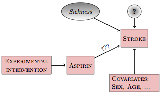
Figure 18.2: Intervening in the aspirin network
Experimental intervention has broken the link between sickness and aspirin since the experimenter, rather than the subject, sets the level of aspirin. There is no longer a backdoor correlating pathway. All the other possibilities for backdoor pathways – e.g., genetics – are also severed. With the experimental intervention, the simple model stroke ~ aspirin is relevant to a wide range of different researchers’ hypothetical causal networks.
Details, however, are important. You need to make sure that the way you assign the values of aspirin to the experimental units doesn’t accidentally create a correlation with other explanatory variables. Techniques for doing this are described in Section 18.6. Another possibility is that your experimental intervention doesn’t entirely set the experimental variable. You can tell the subject how much aspirin to take, but they may not comply! You’ll need to have techniques for dealing with that situation as well. (See Section 18.8.)
18.6 Creating Orthogonality
In setting the experimental intervention, it’s your intention to eliminate any connections between the experimental variables and other variables in the causal network. Doing this requires some care. It’s surprisingly easy to create accidental correlations.
For instance, suppose the person assigning the subjects to either aspirin or placebo thinks it would be best to avoid risk to the sicker people by having them take only the placebo, effectively correlating the treatment with sickness. If such correlations are created, the experimental system will not be so simple: there will still be back doors to be dealt with.
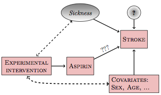
Figure 18.3: If the experimental intervention is influenced by or correlated with other variables in the system, new backdoor pathways will be created.
There are two main ways to avoid accidental correlations: random assignment and blocking.
18.6.1 Random Assignment
In random assignment, you use a formal random process to determine what level of the experimental variable is to be assigned to each experimental unit. When there are just two levels, treatment and control, this can be as simple as flipping a coin. (It’s better to do something that can be documented, such as having a computer generate a list of the experimental units and the corresponding randomly assigned values.)
Random assignment is worth emphasizing, even though it sounds simple:
Random assignment is of fundamental importance.
Randomization is important because it works for any potential
covariate – so long as n is large enough.
Even if there is another
variable that you do not know or cannot measure, your random
assignment will, for large enough n, guarantee that there is no
correlation between your experimental variable and the unknown
variable. If n is small, however, even random assignment may
produce accidental correlations. For example, for n = 25, there’s a
5% chance of the accidental R² being larger than 0.15, whereas
for n=1000, the R² is unlikely to be bigger than 0.005.
Blocking in Experimental Assignment
If you do know the value of a covariate, then it’s possible to do better than randomization at producing orthogonality. The technique is called blocking . The word “blocking” in this context does not refer to disconnecting a causal pathway; it’s a way of assigning values of the experimental variable to the experimental subjects.
To illustrate blocking in assignment, imagine that you are looking at your list of experimental subjects and preparing to assign each of them a value for the experimental variable:
Sex |
Age |
Aspirin |
|---|---|---|
| F | 71 | aspirin |
| F | 70 | placebo |
| F | 69 | placebo |
| F | 65 | aspirin |
| F | 61 | aspirin |
| F | 61 | placebo |
| M | 71 | placebo |
| M | 69 | aspirin |
| M | 67 | aspirin |
| M | 65 | placebo |
Notice that the subjects have been arranged in a particular order and divided into blocks. There are two subjects in each block because there are two experimental conditions: treatment and control. The subjects in each block are similar: same sex, similar age.
Within each block of two, assign one subject to aspirin and the other to placebo. For the purpose of establishing orthogonality of aspirin to sex, it would suffice to make that assignment in any way whatsoever. But since you also want to make aspirin orthogonal to other variables, perhaps unknown, you should do the assignment within each block at random.
The result of doing assignment in this way is that the experimental variable will be balanced : the women will be divided equally between placebo and aspirin, as will the men. This is just another way of saying that the indicator vectors for sex will be orthogonal to the indicator vectors for aspirin.
When there is more than one covariate – the table has both age and sex – the procedure for blocking is more involved. Notice that in the above table, the male-female pairs have been arranged to group people who are similar in age. If the experimental subjects had been such that the two people within each pair had identical ages, then the aspirin assignment would be exactly orthogonal to age and to sex. But because the age variable is not exactly balanced, the orthogonality created by blocking will be only approximate. Still, it’s as good as it’s going to get.
Blocking becomes particularly important when the number of cases n is small. For small n, randomization may not give such good results.
Whenever possible, assign the experimental variable by using blocking against the covariates you think might be relevant, and using randomization within blocks to deal with the potential latent variables and covariates that might be relevant, even if they are not known to you.
Within each block, you are comparing the treatment and control between individuals who are otherwise similar. In an extreme case, you might be able to arrange things so that the individuals are identical. Imagine, for example, that you are studying the effect of background music on student test performance. The obvious experiment is to have some students take the test with music in the background, and others take it with some other background, for instance, quiet.
Better, though, if you can have each student take the test twice: once with the music and once with quiet. Why? Associated with each student is a set of latent variables and covariates. By having the student take the test twice, you can block against these variables. Within each block, randomly assign the student to which background condition to use the first time, with the other background condition being used the second time. This means to pick each student’s assignment at random from a set of assignments that’s balanced: half the students take the test with music first, the other half take the test with quiet first.
18.7 When Experiments are Impossible
Often you can’t do an experiment.
The inability to do an experiment might stem from practical, financial, ethical or legal reasons. Imagine trying to investigate the link between campaign spending and vote outcome by controlling the amount of money candidates have to spend. Where would you get the money to do that? Wouldn’t there be opposition from those candidates who were on the losing side of your random assignment of the experimental variables? Or, suppose you are an economist interested in the effect of gasoline taxes on fuel consumption. It’s hardly possible to set gasoline taxes experimentally in a suitably controlled way. Or, consider how you would do an experiment where you randomly assign people to smoke or to not smoke in order to understand better the link between smoking, cancer, and other illnesses such as emphysema. This can’t be done in an ethical way.
Even when you can do an experiment, circumstances can prevent your setting the experimental variables in the ways that you want. Subjects often don’t comply in taking the pills they have been assigned to take. The families randomly admitted to private schools may decline to go. People drop out in the middle of a study, destroying the balance in your experimental variables. Some of your experimental units might be lost due to sloppy procedures or accidents.
When you can’t do an experiment, you have to rely on modeling techniques to deal with covariates. This means that your assumptions about how the system works – your hypothetical causal networks – play a role. Rather than the data speaking for themselves, they speak with the aid of your assumptions.
Section 18.9 introduces two technical approaches to data analysis that can help to mitigate the impact of your assumptions. This is not to say that the approaches are guaranteed to make your results as valid as they might be if you had been able to do a perfect experiment. Just that they can help. Unfortunately, it can be hard to demonstrate that they actually have helped in any study. Still, even if the approaches cannot recreate the results of an experiment, they can be systematically better than doing your data analysis without using them.
18.8 Intent to Treat
Consider an experiment where the assignment of the experimental variables has not gone perfectly. Although you, the experimenter, appropriately randomized and blocked, the experimental subjects did not always comply with your assignments. Unfortunately, there is often reason to suspect that the compliance itself is related to the outcome of the study. For example, sick subjects might be less likely to take their experimentally assigned aspirin.
A hypothetical causal network describing the imperfect compliance aspirin experiment looks like Figure 18.4, with the value of aspirin determined both by the experimental intervention and the subject’s state of sickness.
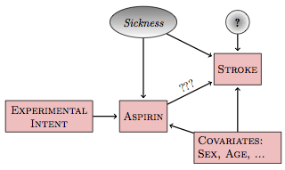
Figure 18.4: In an imperfect experiment, the experimental intent influences the treatment (aspirin, here), but the treatment may be influenced by the covariates and latent variables.
In such a network, the model stroke ~ aspirin describes the total connection between aspirin and stroke. This includes three parts:
- the direct link
aspirin⥤stroke - the backdoor pathway through
sickness - the backdoor pathway through the covariates.
By including the covariates as explanatory variables in your model, you can block pathway (3). The experimental intervention has likely reduced the influence of backdoor pathway (2), but because the subjects may not comply perfectly with your assignment, you cannot be sure that your random assignment has eliminated it.
Consider, now, another possible model: stroke ~ experimental intent. Rather than looking at the actual amount of aspirin that the subject took and relating that to stroke, the explanatory variable is the intent of the experimenter. This intent, however it might have been ignored by the subjects, remains disconnected from any covariates; the intent is the set of values assigned by the experimenter using randomization and blocking in order to avoid any connection with the covariates.
The hypothetical causal network still has three pathways from experimental intent to stroke. One pathway is experimental intent⥤ aspirin⥤ stroke. This is a correlating pathway that subsumes the actual pathway of interest: aspirin⥤ stroke. As such, it’s an important pathway to study, the one that describes the impact of the experimenter’s intent on the subjects’ outcomes.
The other two pathways connecting intent to stroke are the backdoor pathway via sickness and the backdoor pathway via the covariates. These two pathways cause the trouble that the experiment sought to eliminate but that non-compliance by the experimental subjects has re-introduced. Notice, though, that the backdoor pathways connecting experimental intent to stroke are non-correlating rather than correlating. To see why, examine this backdoor pathway:
experimental intent ⥤ aspirin ⥢ sickness ⥤ stroke
There’s no node from which the causal flow reaches both end points. This non-correlating pathway will be blocked so long as sickness is not included in the model. Similarly the back door pathway through the covariates is blocked when the covariates are not included in the model.
As a result, the model stroke ~ experimental intent will describe the causal chain from experimental intent to stroke. This chain reflects the effect of the intent to treat. That chain is not just the biochemical or physiological link between aspirin and stroke, it includes all the other influences that would cause a subject to comply or not with the experimenter’s intent. To a clinician or to a public health official, the intent to treat can be the proper thing to study. It addresses this question: How much will prescribing patients to take aspirin reduce the amount of stroke, taking into account non-compliance by patients with their prescriptions? This is a somewhat different question than would have been answered by a perfect experiment, which would be the effect of aspirin presuming that the patients comply.
Intent to treat analysis can be counter-intuitive. After all, if you’ve measured the actual amount of aspirin that a patient took, it seems obvious that this is a more relevant variable than the experimenter’s intent. That may be, but aspirin is also connected with other variables (sickness and the covariates) which can have a confounding effect. Even though intent is not perfectly correlated with aspirin, it has the great advantage of being uncorrelated with sickness and the covariates – so long as the experimental variables were properly randomized and blocked.
Of course, pure intent is not enough. In order for there to be an actual connection between intent and the outcome variable, some fraction of the patients has to comply with their assignment to aspirin or placebo.
18.9 Destroying Associations
In intent-to-treat analysis, the explanatory variable was changed in order to avoid unwanted correlations between the explanatory variable and covariates and latent variables. The techniques in this section – matched sampling and instrumental variables – allow you to keep your original explanatory variables but instead modify the data in precise ways in order to destroy or reduce those unwanted correlations.
Figure 18.5 shows the general situation. You’re interested in the direct relationship between some treatment and a response, for instance aspirin and stroke. There are some covariates, which might be known or unknown. Also, there can be another variable, an instrumental variable, that is related to the treatment but not directly related to any other variable in the system. An example of an instrumental variable is experimental intent in Figure 18.4, but there can also be instrumental variables relevant to non-experimental systems.
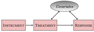
Figure 18.5: An instrument is a variable that is unrelated to the covariates but is connected to the treatment.
A key question for a modeler is how to construct an appropriate model of the relationship between the treatment and the response. The two possibilities are:
response~treatmentresponse~treatment+covariates
The first model is appropriate if the backdoor pathway involving the covariates is a non-correlating pathway; the second model is appropriate if it is a correlating pathway. But it’s not so simple; there can be multiple covariates, some of which are involved in correlating pathways and some not. Beyond that, some of the covariates might be unknown or unmeasured – latent variables – in which case the second form of model isn’t possible; you just don’t have the data.
In a proper experimental design, where you can assign the value of treatment, you use randomization and blocking to arrange treatment to be orthogonal to the covariates. Given such orthogonality, it doesn’t matter whether or not the covariates are included in the model; the coefficient on treatment will be the same either way. That’s the beauty of orthogonality.
In the absence of an experiment, or when the experimental intervention is only partially effective, then treatment will typically not be orthogonal to the covariates. The point of matched sampling and of instrumental variables is to arrange things, by non-experimental means, to make them orthogonal.
Instrumental Variables
An instrumental variable is a variable that is correlated with the treatment variable, but uncorrelated with any of the covariates. Its effect on the response variable, if any, is entirely indirect, via the treatment variable.
Perhaps the simplest kind of instrumental variable to understand is the experimenter’s intent. Assuming that the intent has some effect on the treatment – for instance, that some of the subjects comply with their assigned treatment – then it will be correlated with the treatment. But if the intent has been properly constructed by randomization and blocking, it will be uncorrelated with the covariates. And, the intent ordinarily will affect the response only by means of the treatment. (It’s possible to imagine otherwise, for example, if being assigned to the aspirin group caused people to become anxious, increased their blood pressure, and caused a stroke. Placebos avoid such statistical problems.)
An instrumental variable is orthogonal to the covariates but not to the treatment, and thus it provides a way to restructure the data in order to eliminate the need to include covariates when estimating the relationship between the treatment variable and the response. The approach is very clever but straightforward and is often done in two stages. First, the treatment is projected onto the instrument. The resulting vector is exactly aligned with the instrument and therefore shares the instrument’s orthogonality to the covariates. Second, replace the response by the fitted values of treatment ~ instrument. In doing this, it doesn’t matter whether the covariates are included or not, since they are orthogonal to the projected treatment variable.
If you have an appropriate instrument, the construction of a meaningful model to investigate causation can be straightforward. The challenge is to find an appropriate instrument. For experimenters dealing with imperfections of compliance or drop-out, the experimental intent makes a valid instrument. For others, the issues are more subtle. Often, one looks for an instrument that pre-dates the treatment variable with the idea that the treatment therefore could not have caused the instrument. It’s not the technique of instrumental variables that is difficult, but the work behind it, “the gritty work of finding or creating plausible experiments” (Angrist and Krueger 2001), or the painstaking “shoe-leather” research (Freedman 1991). Finding a good instrumental variable requires detailed understanding of the system under study, not just the data but the mechanisms shaping the explanatory variables.
Imagine, for instance, a study to relate how the duration of schooling relates to earnings after leaving school. There are many potential covariates here. For example, students who do better in school might be inclined to stay longer in school and might also be better earners. Students from low-income families might face financial pressures to drop out of school in order to work, and they might also lack the family connections that could help them get a higher-earning job.
An instrumental variable needs to be something that will be unrelated to the covariates – skill in school, family income, etc. – but will still be related to the duration a student stays in school. Drawing on detailed knowledge of how schools work, researchers Angrist and Krueger (Angrist and Krueger 1991) identified one such variable: date of birth. School laws generally require children to start school in the calendar year in which they turn six and require them to stay in school until their 16th birthday. As a result, school dropouts whose birthday is before the December 31 school-entry cut-off tend to spend more months in school than those whose birthday comes on January 1 or soon after. So date of birth is correlated with duration of schooling. But there’s no reason to think that date of birth is correlated with any covariate such as skill in school or family income. (Angrist and Krueger found that men born in the first quarter of the calendar year had about one-tenth of a year less schooling than men born in the last quarter of the year. The first-quarter men made about 0.1 percent less than the last-quarter men. Comparing the two differences indicates that a year of schooling leads to an increase in earnings of about 10%.)
Matched Sampling
In matched sampling, you use only a subset of your data set. The subset is selected carefully so that the treatment is roughly orthogonal to covariates. This does not eliminate the actual causal connection between the treatment and the covariates, but when fitting a model to the subset of the data, the coefficient on treatment is rendered less sensitive to whether the covariates are included in the model.
To illustrate, imagine doing an observational study on the link between aspirin and stroke. Perhaps you pick as a sampling frame all the patients at a clinic ten years previously, looking through their medical records to see if their physician has asked them to take aspirin in order to prevent stroke, and recording the patients age, sex, and systolic blood pressure. The response variable is whether or not the patient has had a stroke since then. The data might look like this:
| Case # | Aspirin Recommended | Age | Sex | Systolic Blood Pressure | Had a Stroke |
|---|---|---|---|---|---|
| 1 | Yes | 65 | M | 135 | Yes |
| 2 | Yes | 71 | M | 130 | Yes |
| 3 | Yes | 68 | F | 125 | No |
| 4 | Yes | 73 | M | 140 | Yes |
| 5 | Yes | 64 | F | 120 | No |
| … and | so on | … | |||
| 101 | No | 61 | F | 110 | No |
| 102 | No | 65 | F | 115 | No |
| 103 | No | 72 | M | 130 | No |
| 104 | No | 63 | M | 125 | No |
| 105 | No | 64 | F | 120 | No |
| 106 | No | 60 | F | 110 | Yes |
| … and | so on | … |
Looking at these data, you can see there is a relationship between aspirin and stroke – the patients for whom aspirin was recommended were more likely to have a stroke. On the other hand, there are covariates of age, sex, and blood pressure. You might also notice that the patients who were recommended to take aspirin typically had higher blood pressures. That might have been what guided the physician to make the recommendation. In other words, the covariate blood pressure is aligned with the treatment aspirin. The two groups – aspirin or not – are different in other ways as well: the no-aspirin group is more heavily female and younger.
To construct a matched sample, select out those cases from each group that have a closely matching counterpart in the other group. For instance, out of the small data set given in the table, you might pick these matched samples:
| Case # | Aspirin Recommended | Age | Sex | Systolic Blood Pressure | Had a Stroke |
|---|---|---|---|---|---|
| 5 | Yes | 64 | F | 120 | No |
| 105 | No | 64 | F | 120 | No |
| 2 | Yes | 71 | M | 130 | Yes |
| 103 | No | 72 | M | 130 | No |
The corresponding pairs (cases #5 and #105, and cases #2 and #103) match closely according to the covariates, but each pair is divided between the values of the treatment variable, aspirin. By constructing a subsample in this way, the covariates are made roughly orthogonal to the treatment. For example, in the matched sample, it’s not true that the patients who were recommended to take aspirin have a higher typical blood pressure.
In a real study, of course, the matched sample would be constructed to be much longer – ideally enough data in the matched sample so that the power of the study will be large.
There is a rich variety of methods for constructing a matched sample. The process can be computationally intensive, but is very feasible on modern computers. Limits to practicality come mainly from the number of covariates. When there is a large number of covariates, it can be hard to find closely matching cases between the two treatment groups.
A powerful technique involves fitting a propensity score, which is the probability that a case will be included in the treatment group (in this example, aspirin recommended) as a function of the covariates. (This probability can be estimated by logistic regression.) Then matching can be done simply using the propensity score itself. This does not necessarily pick matches where all the covariates are close, but is considered to be an effective way to produce approximate orthogonality between the set of covariates and the treatment.
Example: Returning to Campaign Spending …
Analysis of campaign spending in the political science literature is much more sophisticated than the simple model vote ~ spending. Among other things, it involves consideration of several covariates to try to capture the competitiveness of the race. An influential series of papers by Gary Jacobson (e.g., (Jacobson 1978,jacobson-1990)) considered, in addition to campaign spending by the incumbent and vote outcome, measures of the strength of the challenger’s party nationally, the challenger’s expenditures, whether the challenger held public office, the number of years that the incumbent has been in office, etc. Even including these covariates, Jacobson’s least-square models showed a much smaller impact of incumbent spending than challenger spending. Based on the model coefficients, a challenger who spends $100,000 will increase his or her vote total by about 5 percent, but an incumbent spending $100,000 will typically increase the incumbent’s share of the vote by less than one percent.
In order to deal with the possible connections between the covariates and spending, political scientists have used instrumental variables. (The term found in the literature is sometimes two-stage least squares as opposed to instrumental variables.) Green and Krasno (Green and Krasno 1988), in studying elections to the US House of Representatives in 1978, used as an instrument incumbent campaign expenditures during the 1976 election. The idea is that the 1976 expenditures reflects the incument’s propensity to spend, but expenditures in 1976 could not have been caused by the situation in 1978. When using this instrument, Green and Krasno found that $100,000 in incumbent expenditures increased his or her vote total by about 3.7 percent – much higher than the least squares model constructed without the instrument. (Jacobson’s reports also included use of instrumental variables, but his instruments were too collinear and insufficiently correlated with spending to produce stable results.)
Steven Levitt (whose later book Freakonomics (Levitt and Dubner 2005) became a best-seller) took a different perspective on the problem of covariates: matched sampling. (Or, to use the term in the paper, panel data.) He looked at the elections to the US House between 1972 and 1990 in which the same two candidates – incumbent and challenger – faced one another two or more times. This was only about 15% of the total number of House elections during the period, but it is a subset where the covariates of candidate quality or personality are held constant for each pair. Levitt found that the effect of spending on vote outcome was small for both challengers and incumbents: an additional $100,000 of spending is associated with a 0.3 percent vote increase for the challenger and 0.1 percent for the incumbent – neither spending effect was statistically significant in an F test.
So which is it? The different modeling approaches give different results. Jacobson’s original work indicates that challenger spending is effective but not incumbent spending; Green and Krasno’s instrumental variable approach suggests that spending is effective for both candidates; Levitt’s matched sampling methodology signals that spending is ineffective for both challenger and incumbent. The dispute focuses attention on the validity of the instruments or the ability of the matching to compensate for changing covariates. Is 1976 spending a good instrument for 1978 elections? Is the identity of the candidates really a good matching indicator for all the covariates or lurking variables? Such questions can be challenging to answer reliably. If only it were possible to do an experiment!
18.10 Conclusion
It’s understandable that people are tempted to use correlation as a substitute for causation. It’s easy to calculate a correlation: Plug in the data and go! Unfortunately, correlations can easily mislead. As in Simpson’s paradox, the results you get depend on what explanatory variables you choose to include in your models.
To draw meaningful conclusions about causation requires work. At a minimum, you have to be explicit about your beliefs about the network of connections and examine which potential explanatory variables lie on correlating pathways and which on non-correlating pathways. If you do this properly, your modeling results can be correctly interpreted in the context of your beliefs. But if your beliefs are wrong, or if they are not shared by the people who are reading your work, then the results may not be useful. There’s room for disagreement when it comes to causation because reasonable people can disagree about the validity of assumptions.
Other analysis techniques – for instance matched sampling or instrumental variables – can ease the dependence of your results on your assumptions and beliefs. But still there is room for interpretation. Is the instrument really uncorrelated with the covariates? How complete is the set of covariates included in your matched sampling?
Ultimately, for a claim about causation to be accepted by skeptics, you need to be able to demonstrate that your assumptions are true. This can be particularly challenging when the skeptics have to take statistical methodology on faith. You’ll find that many decision makers have little or no understanding of methodology, and some critics are willfully ignorant of statistics. On the other hand, it’s appropriate for the modeler to show some humility and to work honestly to identify those assumptions that are not themselves adequately justified by the data, problems with the sampling process, and the potential mis-interpretation of p-values. A good experiment can be invaluable, since the experimenter herself determines the structure of the system and since the statistical analysis can be straightforward.
It’s sometimes said that science is a process of investigation, not a result. The same is true for statistical models. Each insight that is demonstrably supported by data becomes the basis for refinement in the way you collect new data, the variables and covariates you measure in future work, the incisive experimental interventions that require labor, resources, and expertise. However well your data have been collected and your models have been structured and built, the conclusions drawn from statistical models are still inductive, not deductive.
As such, they are not certain. Even so, they can be useful.