Models that learn
Learning and Intelligence
“Machine learning” and “artificial intelligence” are phrases closely associated with computer services and prognoses for future development. (The term “statistical learning” which covers the same territory1, has not been as popular.)
“Learning” and “intelligence” have a sort of mystery about them. If we are to be informed consumers of ML and AI products, we should try to take away some of the mystery. For example, the COMPAS system–Correctional Offender Management Profiling for Alternative Sanctions–has built-in biases reflecting the way that training data is acquired. It’s also an example of how technical ignorance hobbles meaningful evaluation of performance. (In the case of COMPAS, the decision makers often don’t know that “accuracy” is not a good measure of performance and to look instead at “sensitivity” and “specificity” with awareness of the trade-offs between them.)
Simple ML–Classification and Regression Trees
The method of recursive partitioning
In this example, we work with some data about the sales and prices of child car seats. The data come from the ISLR package: a data table Carseats.
The data
Companies generally hold sales and marketing data confidential. This leads to an unfortunate situation for students and educators; realistic data is not readily available for the purposes of teaching and practice. The Carseats data has been generated from a simulation.
Graphic:

Can you see:
- a relationship between sales and price?
- a relationship between population and sales?
- a relationship between competitor’s price and sales of your product?
Could you convince your (imagined) product manager of the importance or unimportance of these relationships?
Quantitative presentations:
Linear Modeling
Linear modeling to produce coefficients and confidence intervals. This is perhaps the earliest machine learning technique. (But it’s usually not classified as “machine learning.” If it had been invented in 2010 instead of 1910, it would earn the label “machine learning.”)
##
## Call:
## lm(formula = Sales ~ Price + Population + CompPrice, data = Carseats)
##
## Residuals:
##     Min      1Q  Median      3Q     Max
## -5.4920 -1.5940 -0.2328  1.6072  6.0576
##
## Coefficients:
##               Estimate Std. Error t value Pr(>|t|)
## (Intercept)  5.6328747  0.9727948   5.790 1.43e-08 ***
## Price       -0.0881579  0.0058936 -14.958  < 2e-16 ***
## Population   0.0017113  0.0007715   2.218   0.0271 *
## CompPrice    0.0929665  0.0091402  10.171  < 2e-16 ***
## ---
## Signif. codes:  0 '***' 0.001 '**' 0.01 '*' 0.05 '.' 0.1 ' ' 1
##
## Residual standard error: 2.258 on 396 degrees of freedom
## Multiple R-squared:  0.3657, Adjusted R-squared:  0.3609
## F-statistic: 76.11 on 3 and 396 DF,  p-value: < 2.2e-16
## Analysis of Variance Table
##
## Response: Sales
## Df Sum Sq Mean Sq F value Pr(>F)
## Price 1 630.03 630.03 123.6044 <2e-16 ***
## Population 1 6.46 6.46 1.2682 0.2608
## CompPrice 1 527.31 527.31 103.4514 <2e-16 ***
## Residuals 396 2018.47 5.10
## ---
## Signif. codes: 0 '***' 0.001 '**' 0.01 '*' 0.05 '.' 0.1 ' ' 1Displaying the model:

How would you re-arrange the variables to make the effect (or lack of effect) of each variable clear?
Regression tree
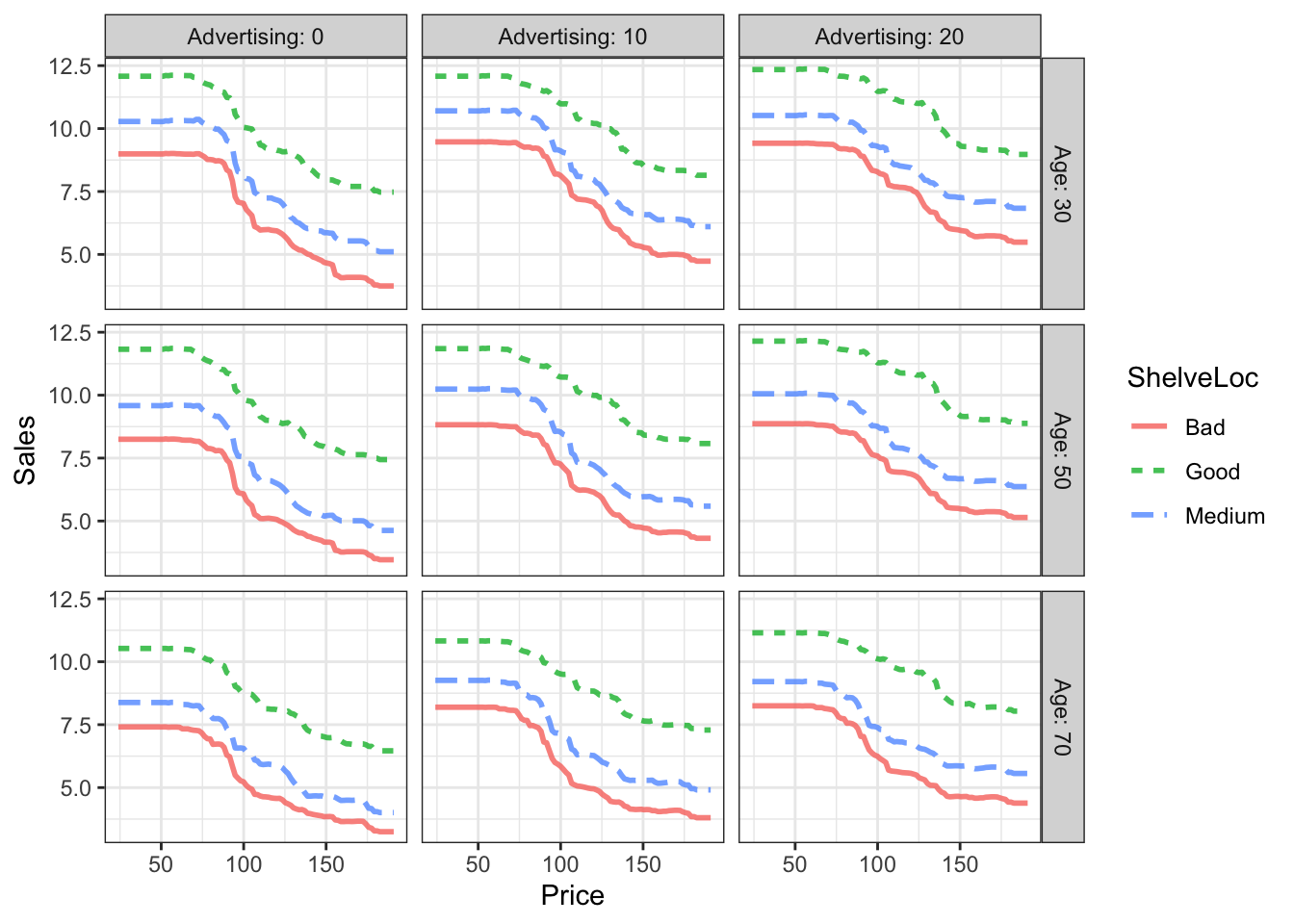
An middle-aged machine-learning technique


Things to note from the graphical model:
- Advertising doesn’t matter, except for high levels of advertising with the product in a “good” shelf location.
- In general, people will look at bad shelf locations if the price is low.
- Old people won’t reach down to the lower shelf even if the price is low.
Random Forest
An newish machine-learning technique
##             IncNodePurity
## CompPrice       287.95073
## Income          233.79034
## Advertising     267.96635
## Population      192.50218
## Price           746.90476
## ShelveLoc       775.71585
## Age             332.65234
## Education       127.76003
## Urban            23.61308
## US               41.12407
A more nuanced relationship between price and sales and between shelf location and sales.
Predicting survival from the Titanic
From USCOTS short course.
AI started out focussed on different techniques such as rule-based reasoning, but the label has been applied more and more to techniques that are statistical in nature. But statistics itself has been influenced by AI, as with Judea Pearl’s bayesian networks from which emerged his work on causality.↩