A Confounding Interval
As part of the pedagogy of “association is not causation,” some bogeyman phrases are used, among which “confounding” or “lurking” variables.
The adjective lurking is clearly about a threat. Here’s a dictionary definition:
remaining hidden so as to wait in ambush. “the trumpet fish is a lurking predator”
(of an unpleasant quality) present in a latent or barely discernible state, although still presenting a threat. “he lives with a lurking fear of exposure as a fraud”
Confounding has a similarly negative connotation. The leading dictionary definition is:
cause surprise or confusion in (someone), especially by acting against their expectations.
But for teaching people about statistics (as opposed to scaring them), it’s better to go back to the origins of the word and the reason why it’s an appropriate technical term. The second dictionary definition does this:
mix up (something) with something else so that the individual elements become difficult to distinguish. from Old French confondre, from Latin confundere ‘pour together, mix up’.
The statistical and mathematical methods for unmixing are central to responsible professional work in statistics. Unmixing is most often attempted by multiple regression.
In my Statistical Modeling: A Fresh Approach I tried to demonstrate how multiple regression can be a good basis for introductory statistics. Still, this view has not come to be universally accepted, especially for instructors reluctant to use modern computing. And so how do we help students to approach confounding with confidence and to distinguish between the situations where it is an overwhelming problem and when it’s not.
A mathematically tractable problem
When students are limited to techniques such as simple regression or the t-test that have only one explanatory variable, we don’t give them a way to confront confounding. And, really, what can you say about confounding without introducing real-world knowledge about the various factors that can influence an outcome? Actually, quite a bit.
This was demonstrated first, perhaps, around 1960 by Jerome Cornfield, then at the NIH. The setting was important: the debate about whether smoking causes cancer. Famous statisticians (who, incidentally, were smokers, like so many of their generation) pointed out that there could be confounding involved in the observed association between smoking and cancer. For instance, Fisher proposed that there might be a genetic factor that was the common cause of both smoking and cancer. (Fisher was the founder of the genetics department at Cambridge, perhaps putting some authority behind his otherwise unsupported statement.)
Cornfield showed that the strength of the observed relationship between smoking and cancer would require the hypothesized common cause to be extremely strong: indeed the genetic factor would have to have a correlation that was implausibly deterministic of both cancer and smoking. Cornfield’s argument put an end to Fisher’s hypothesis, an important step leading up to the hugely influential 1964 US Surgeon General’s report on smoking and cancer.
One way to get a handle on possible confounding without data is to estimate the plausible level of correlation between a confounding variable and (1) the explanatory variable (e.g. smoking) and the (2) response variable (e.g. cancer).
As it happens, Fisher introduced in the 1910’s a novel way of looking at statistics involving vectors in high-dimensional space. The space is defined to have one dimension for each unit of observation. In this space, a variable corresponds to a single vector.
Correlation between two variables amounts to an alignment between the two corresponding vectors. Indeed, the correlation coefficient is the cosine of the angle between the two vectors.
If you imagine a covariate with a given strength of correlation with the response variable, that covariate’s vector must lie in a (hyper-) cone subtended by the given angle around the response variable. Similarly, the correlation of the explanatory variable with the covariate implies that the covariate lies simultaneously in a cone about the explanatory variable. These two cones put a constraint on the possible angles between the response and explanatory variable. By considering the range of positions of the three vectors–response, explanatory, covariate–one can figure out a range of expected results if the covariate had been measured and used in a multiple regression.
I have made an attempt to solve this geometrical problem. (Someone with more mathematical insight could probably do a better job.) I’ve summarized the range of possibilities into an interval, which I call the confounding interval.
The diagram siows the confounding interval as a function of the strength of correlation between the response and explanatory variable, and a hypothesized strength of correlation between the covariate and each of the response and explanatory variables individually.
Shown in the graph is the range within which the effect size is uncertain due to the hypothesized confounding. The confounding interval is very wide when there is strong correlation between the confounder and the response and explanatory variable, particularly when the correlation between the response and explanatory variables themselves is week.
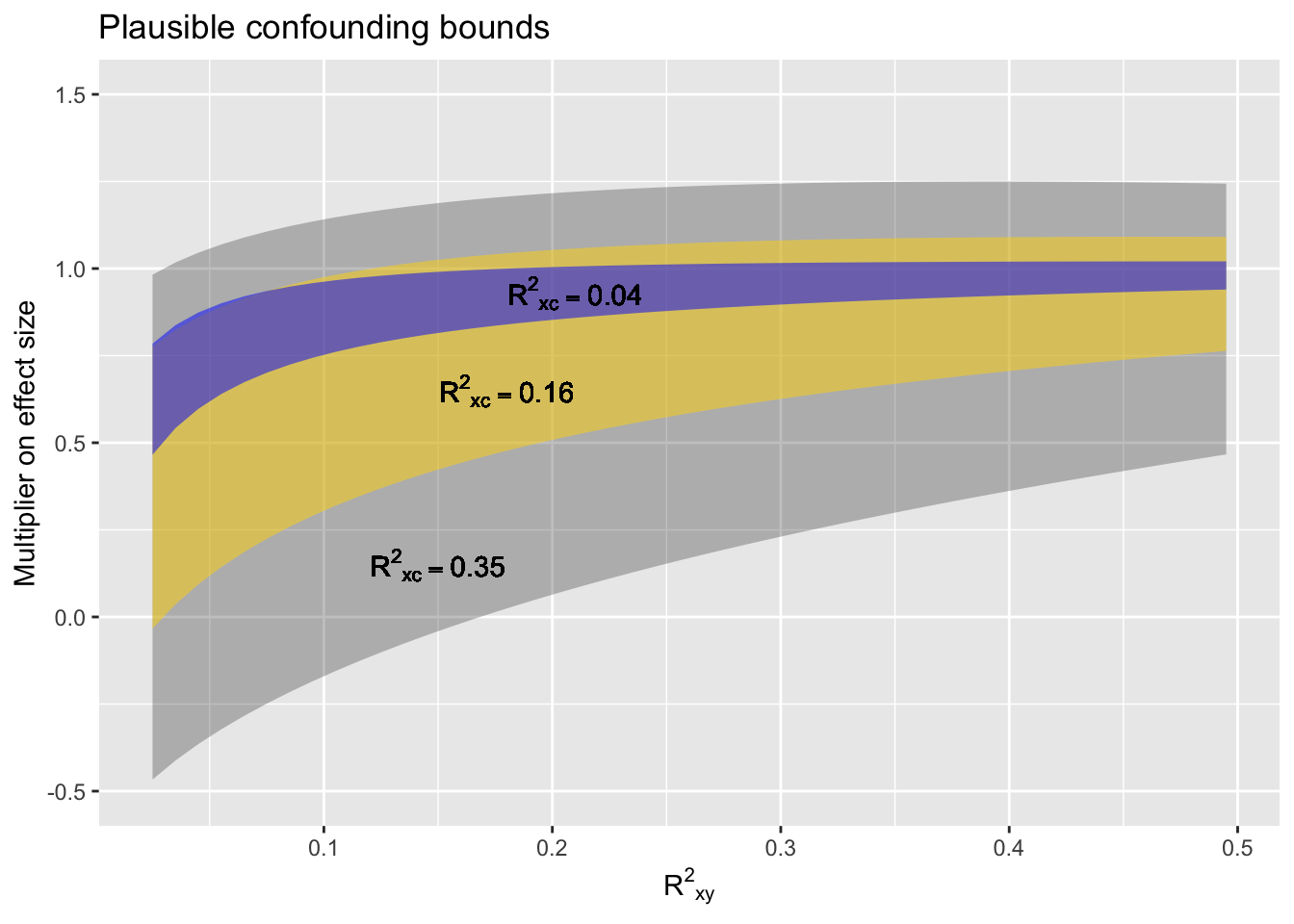
Note that the confounding interval does not depend on the sample size n. It is not about sampling variation, it is about the possible arrangements of the three vectors involved. For large n, the confounding interval is going to swamp the confidence interval.
To use the confounding interval,
- Calculate the correlation between the response and explanatory variable.
- Hypothesize how strongly the confounder might be correlated with the response and explanatory variables.
- Look up the corresponding interval on the graph. That interval is a multiplier on the effect size. When the interval includes values below zero, Simpson’s paradox is potentially an issue.
A proposed policy
- Did a perfect experiment? No need for plausible confounding bounds.
- Did a real experiment? Use weak plausible confounding bounds.
- Know a lot about the system you’re observing and confident that the significant confounders have been adjusted for? Use weak plausible confounding bounds.
- Not sure what all the confounders might be, but controlled for the ones you know about? Use moderate plausible confounding bounds.
- Got some data and you want to use it to figure out the relationship between X and Y? Use strong plausible confounding bounds.
The confounding interval is about how concerned you should be about possible confounders. If the interval is very broad, you should lack confidence in the face value of the observed relationship between the response and explanatory variables, even if the confidence interval is narrow.