Generalizing Inference
Objectives: Cover the genuinely useful settings of a traditional intro stats course while …
- saving time, so that we can choose to cover other topics: e.g. covariation, causality, decision-making, …
- setting things up for more advanced settings: multiple regression, machine learning models, classification, …
- simplifying the framework
- one set of formulas
- simple (or trivial) critical values
- avoiding undue emphasis on p values
- keeping an emphasis on prediction
Recap:
- Make graphics about data, with annotations always presented in the context of data.
- Rather than calculating “statistics” (e.g. mean, medians, …) build a prediction model
- Focus on effect size in natural units rather than dimensionless quantities such as r or \(\chi^2\) or \(p\).
Now … how to set up the inference calculations.
Variance: How much variation?
We focus on the response variable …
Average pairwise square differences between values.
\[\frac{1}{n (n-1)}\sum_{i \neq j} |x_i - x_j|^2 = 2\ \mbox{Var}(x)\]
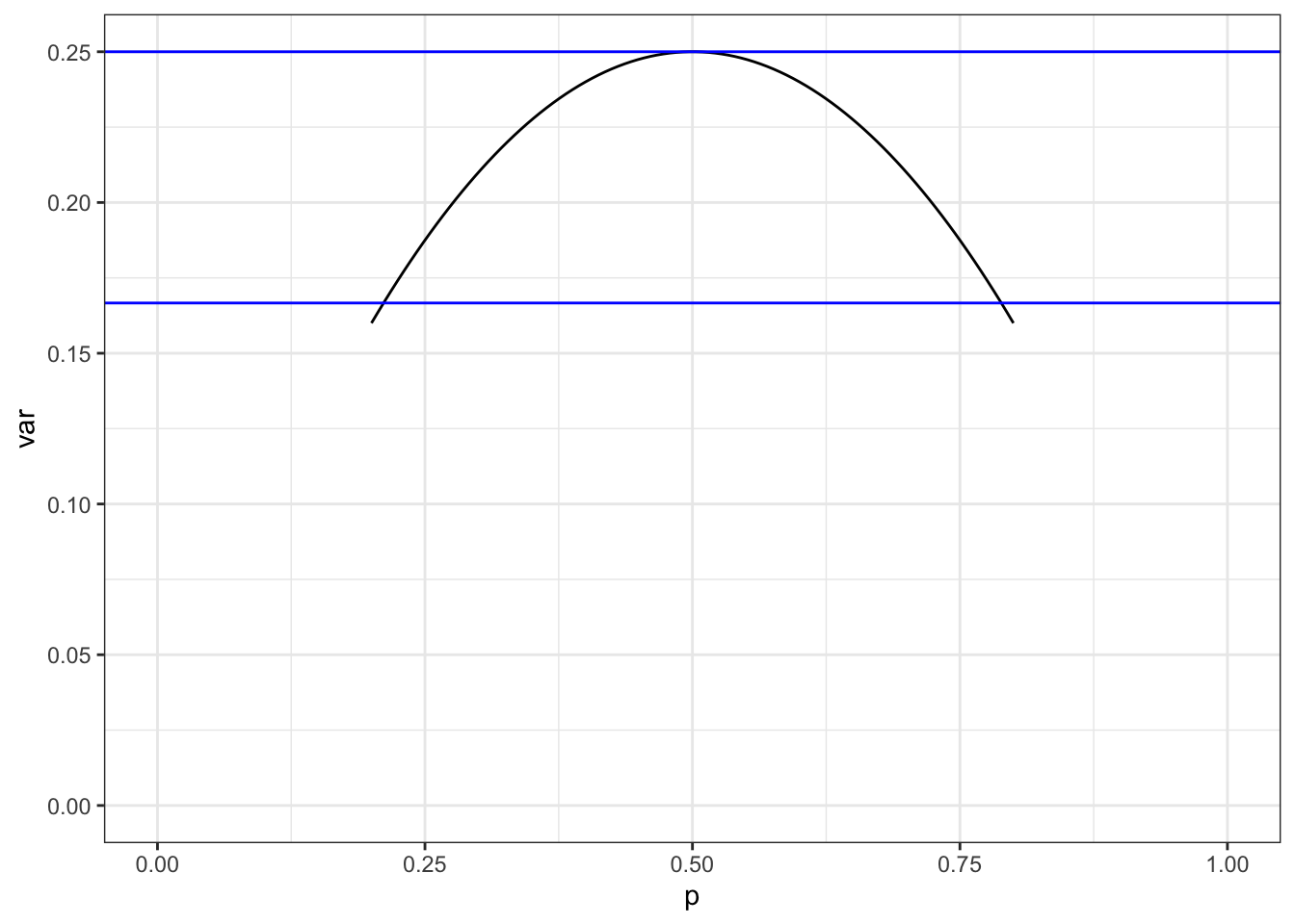
Estimating variance by eye:
- more-or-less normal: find interval covering the central 2/3 of the data. (Thus, 1/6 is left out at either end.) Divide by 2 and square to get the variance.
- Two discrete levels: \(\Delta^2 p(1-p)\)
- \(p (1-p) \approx 1/4\) when levels are more or less equally populated
- \(p (1-p) \approx 1/6\) when levels are noticeably unequally populated.
Model values: How much has been explained?

Basic discernibility
Note that I’m being much more mathy here than I would in teaching a typical class. The audience here is professional mathematicians, hence likely not too scared by algebraic notation.
- Is there any discernible relationship between the response and explanatory variables revealed by the model?
- Inputs from the model: \(v_r\), \(v_m\), \(n\), and degrees of flexibility \(^\circ{\cal F}\)
- Output: \[\mbox{F} = \frac{n - (^\circ{\cal F} + 1)}{^\circ{\cal F}} \frac{v_m}{v_r - v_m}\] … or, equivalently, … \[\mbox{F} = \frac{n - (^\circ{\cal F} + 1)}{^\circ{\cal F}} \frac{R^2}{1 - R^2}\]
- Interpretation: Is F \(\gtrapprox 4\)?. Then a relationship is discernible.
Confidence intervals (when \(^\circ\!{\cal F} = 1\))
When \(^\circ\!{\cal F} = 1\), there is only one explanatory variable and the modeling situation is one of these:
- difference between two groups
- slope of a regression line
Either way, there is only one effect size: the difference or slope.
- Inputs:
- Effect size B
- F
- Output:
- Margin of error is \(\pm \mbox{B} \sqrt{4 / \mbox{F}}\)
- Interpretation:
- We wouldn’t be at all surprised if a much, much bigger study revealed an effect size within the confidence interval. - If we are comparing our study to another study, we’re only justified in claiming a contradiction when the two confidence intervals don’t overlap.
- Do we really need to refer to populations?
Note that when \(^\circ\!{\cal F} \geq 2\), there is either more than one explanatory variable or more than one group in that explanatory variable or a non-straight-line regression (e.g. a polynomial). In none of these cases can the margin of error be deduced directly from F due to one or more of:
- effect size not constant
- multiple effect sizes
- collinearity among explanatory variables
Instead of the simple formula based on F, confidence intervals can be based on a regression table or bootstrapping.
Activity 3
See the handout on R2 showing the same settings as in the previous chapters. You should already have estimated an effect size of the response with respect to the x-axis variable.
- Estimate R2. Hint: This should be easy, though you have to remember to square.
- Pick a few settings of interest. For each:
- Do a significance test using F.
- For settings with \(^\circ\!{\cal F} = 1\), calculate a 95% confidence interval on the effect size.
Standard statistical calculations
We revisit the settings on the handout, showing the F calculation and a standard statistical report.
Setting A: Difference in two proportions 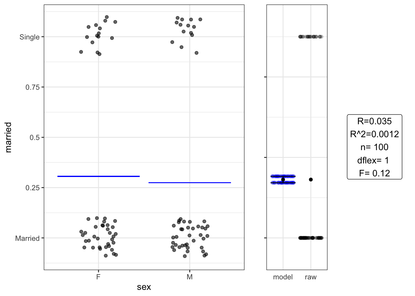
##             Estimate Std. Error t value Pr(>|t|)
## (Intercept)    0.310      0.065    4.70  9.3e-06
## sexM          -0.032      0.092   -0.34  7.3e-01
## Analysis of Variance Table
##
## Response: married
## Df Sum Sq Mean Sq F value Pr(>F)
## sex 1 0.025 0.024974 0.119 0.7308
## Residuals 98 20.565 0.209847No relationship discernable. How much data should we plan for in a repeat study?
Setting B: Difference in two means 
##             Estimate Std. Error t value Pr(>|t|)
## (Intercept)      9.6       0.61   16.00  7.7e-29
## unionUnion       1.1       1.30    0.82  4.1e-01
## Analysis of Variance Table
##
## Response: wage
## Df Sum Sq Mean Sq F value Pr(>F)
## union 1 19.44 19.439 0.672 0.4144
## Residuals 98 2834.98 28.928Setting D : Slope of a regression line 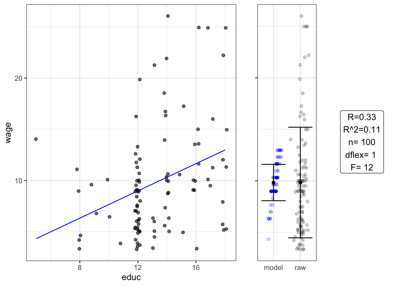
##             Estimate Std. Error t value Pr(>|t|)
## (Intercept)     1.00       2.60    0.39  0.70000
## educ            0.66       0.19    3.40  0.00084
## Analysis of Variance Table
##
## Response: wage
## Df Sum Sq Mean Sq F value Pr(>F)
## educ 1 308.54 308.537 11.877 0.0008386 ***
## Residuals 98 2545.89 25.978
## ---
## Signif. codes: 0 '***' 0.001 '**' 0.01 '*' 0.05 '.' 0.1 ' ' 1Setting H Gets at same thing as chi-squared test 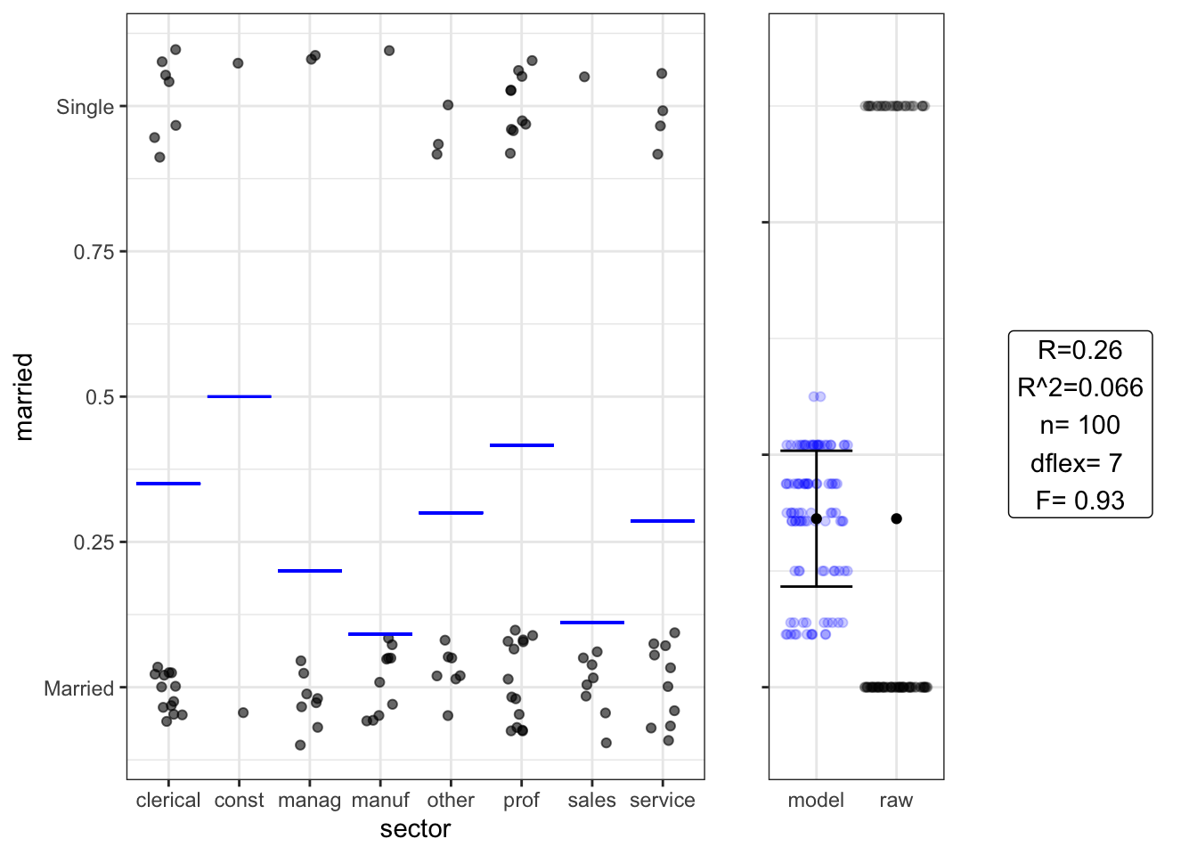
##               Estimate Std. Error t value Pr(>|t|)
## (Intercept)      0.350       0.10    3.40  0.00093
## sectorconst      0.150       0.34    0.44  0.66000
## sectormanag     -0.150       0.18   -0.85  0.40000
## sectormanuf     -0.260       0.17   -1.50  0.13000
## sectorother     -0.050       0.18   -0.28  0.78000
## sectorprof       0.067       0.14    0.48  0.63000
## sectorsales     -0.240       0.18   -1.30  0.20000
## sectorservice   -0.064       0.16   -0.40  0.69000
## Analysis of Variance Table
##
## Response: married
## Df Sum Sq Mean Sq F value Pr(>F)
## sector 7 1.3515 0.19308 0.9233 0.4924
## Residuals 92 19.2385 0.20911Not so often reached in intro stats
Setting I: “One-way” ANOVA 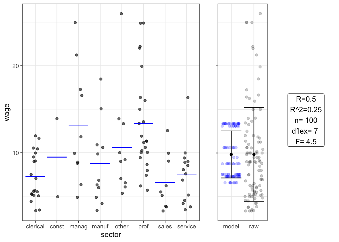
##               Estimate Std. Error t value Pr(>|t|)
## (Intercept)       7.30        1.1    6.80  1.2e-09
## sectorconst       2.20        3.6    0.62  5.4e-01
## sectormanag       5.80        1.9    3.10  2.5e-03
## sectormanuf       1.50        1.8    0.82  4.2e-01
## sectorother       3.30        1.9    1.80  7.8e-02
## sectorprof        6.10        1.5    4.20  7.0e-05
## sectorsales      -0.70        1.9   -0.36  7.2e-01
## sectorservice     0.27        1.7    0.16  8.7e-01
## Analysis of Variance Table
##
## Response: wage
## Df Sum Sq Mean Sq F value Pr(>F)
## sector 7 720.4 102.915 4.4368 0.000275 ***
## Residuals 92 2134.0 23.196
## ---
## Signif. codes: 0 '***' 0.001 '**' 0.01 '*' 0.05 '.' 0.1 ' ' 1Setting F “Two-way” ANOVA: wage ~ educ * sex 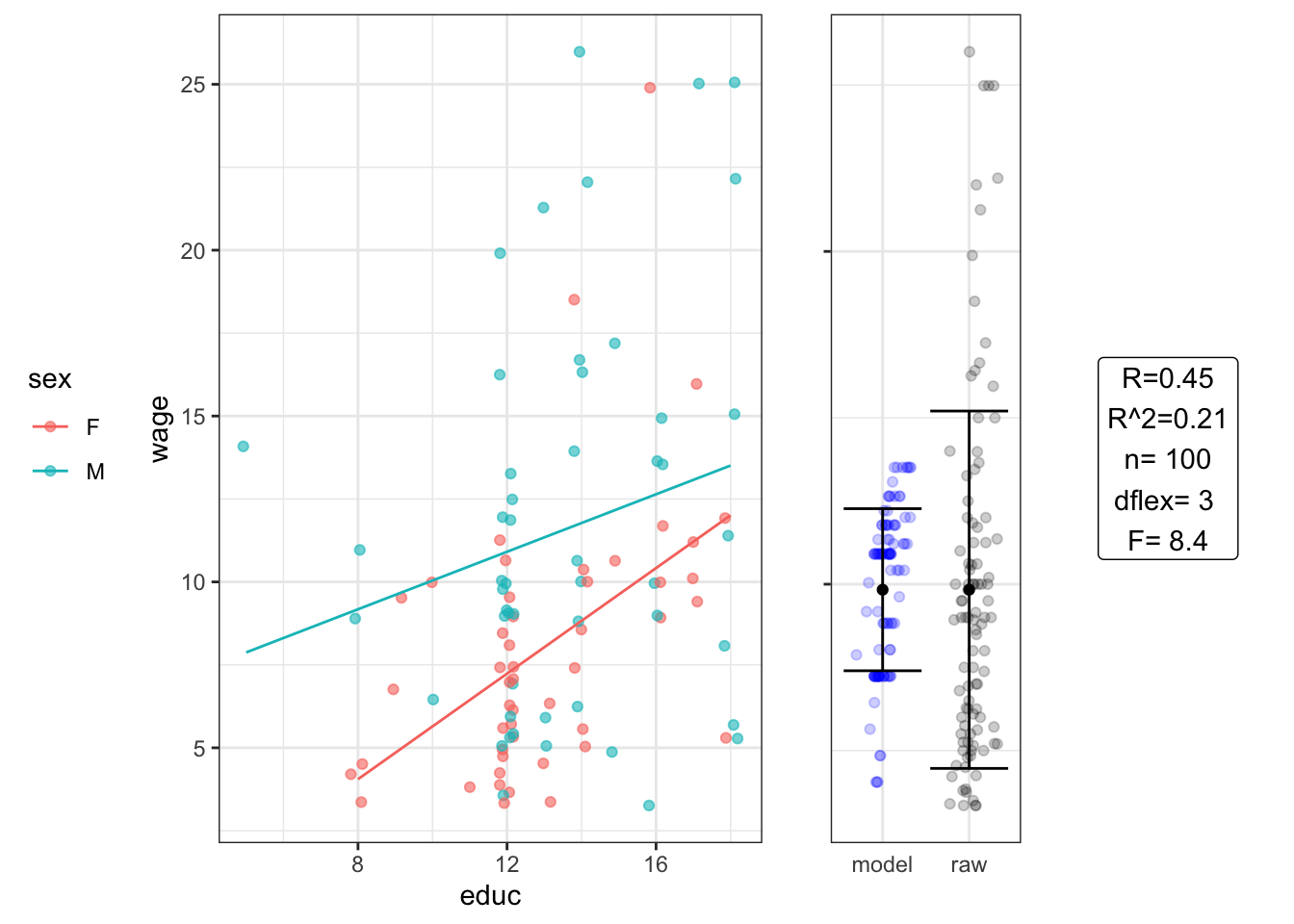
##             Estimate Std. Error t value Pr(>|t|)
## (Intercept)    -2.30       3.70   -0.63   0.5300
## educ            0.80       0.28    2.80   0.0054
## sexM            8.00       5.00    1.60   0.1100
## educ:sexM      -0.36       0.37   -0.97   0.3300
## Analysis of Variance Table
##
## Response: wage
## Df Sum Sq Mean Sq F value Pr(>F)
## educ 1 308.54 308.537 13.0642 0.0004816 ***
## sex 1 256.42 256.421 10.8575 0.0013793 **
## educ:sex 1 22.23 22.231 0.9413 0.3343837
## Residuals 96 2267.23 23.617
## ---
## Signif. codes: 0 '***' 0.001 '**' 0.01 '*' 0.05 '.' 0.1 ' ' 1Need to compare to results from wage ~ educ + sex
Setting J ANCOVA 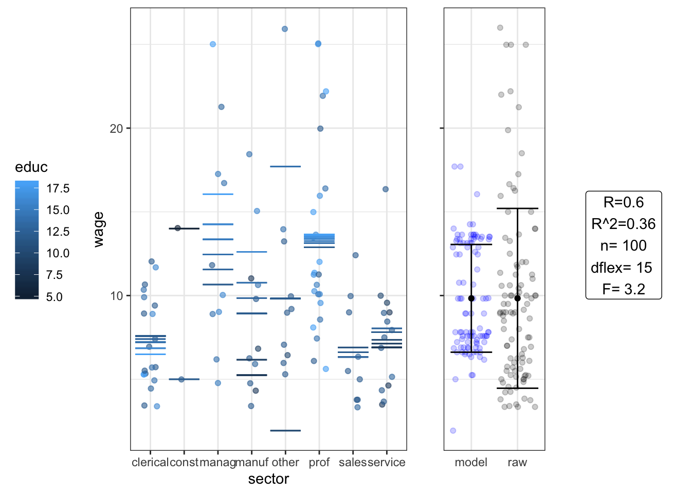
##                    Estimate Std. Error t value Pr(>|t|)
## (Intercept)            9.80       7.10  1.4000    0.170
## sectorconst           11.00      11.00  0.9500    0.340
## sectormanag           -9.90      15.00 -0.6500    0.520
## sectormanuf          -12.00       9.90 -1.2000    0.230
## sectorother          -47.00      18.00 -2.6000    0.011
## sectorprof             1.60      10.00  0.1600    0.880
## sectorsales            0.27      34.00  0.0078    0.990
## sectorservice         -4.70      11.00 -0.4500    0.660
## educ                  -0.18       0.51 -0.3500    0.720
## sectorconst:educ      -1.10       1.10 -1.0000    0.310
## sectormanag:educ       1.10       1.00  1.0000    0.310
## sectormanuf:educ       1.10       0.77  1.4000    0.160
## sectorother:educ       4.10       1.50  2.8000    0.006
## sectorprof:educ        0.31       0.70  0.4400    0.660
## sectorsales:educ      -0.10       2.80 -0.0370    0.970
## sectorservice:educ     0.41       0.87  0.4700    0.640
## Analysis of Variance Table
##
## Response: wage
## Df Sum Sq Mean Sq F value Pr(>F)
## sector 7 720.40 102.915 4.7248 0.000165 ***
## educ 1 30.84 30.836 1.4157 0.237468
## sector:educ 7 273.53 39.076 1.7940 0.099104 .
## Residuals 84 1829.66 21.782
## ---
## Signif. codes: 0 '***' 0.001 '**' 0.01 '*' 0.05 '.' 0.1 ' ' 1No relationship is discernable. How big an n should we have if we want to have a high likelihood of detecting a relationship? (Hint: We want F > 4.)
Setting G: Accomplishes the same as Three-variable chi-squared: married ~ sex * union 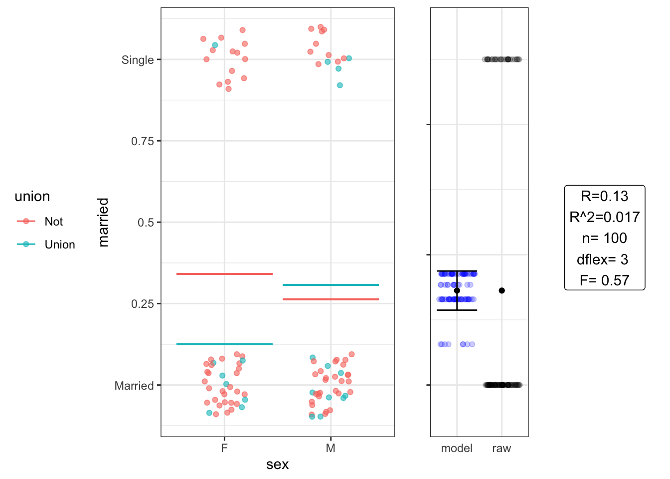
##                 Estimate Std. Error t value Pr(>|t|)
## (Intercept)        0.340      0.072    4.80  6.8e-06
## sexM              -0.078      0.100   -0.76  4.5e-01
## unionUnion        -0.220      0.180   -1.20  2.3e-01
## sexM:unionUnion    0.260      0.230    1.10  2.6e-01
## Analysis of Variance Table
##
## Response: married
## Df Sum Sq Mean Sq F value Pr(>F)
## sex 1 0.0250 0.024974 0.1185 0.7314
## union 1 0.0632 0.063218 0.3000 0.5852
## sex:union 1 0.2696 0.269644 1.2794 0.2608
## Residuals 96 20.2322 0.210752