6 Hypothetical reasoning & Bayes
computing
R
Remember to hand in your work …
At any point, you can submit your answers by collecting them and uploading them to the class site.
No answers yet collected
If the answers that have been loaded automatically are not yours, press this button before starting your work:
6.1 Objectives
Understand the basic components and vocabulary of the Bayesian framework: “relative probability,” “prior probability,” “likelihoods,” “posterior probability,” and “updating belief based on data.”
Be aware of the dominant (but flawed) paradigm of “hypothesis testing” and how it corresponds to a Bayesian calculation but with some essential components deleted.
Know what a “p-value” is and be aware of highly prevalent misconceptions about it. Know what additional information to ask for to put a p-value in proper context.
6.2 Introduction
This tutorial is about the Bayesian framework for evaluating competing hypotheses. To start, consider this simple, general definition of “hypothesis”:
Hypothesis: A statement about the world that might or might not be true.
A detective investigating a crime has suspects. Each of the suspects (or someone else entirely) might be the culprit. In detective novels you read statements like these: “the Butler did it,” or “the nephew is guilty.” Any such statement might or might not be true; they are all hypotheses. The action of detective novels revolves around the collection of new observations or the discovery of facts: footsteps in the garden bed, a dirty shovel in the shed, a suspect running away. Each such observation or fact can have an effect on the level of suspicion of one or more suspects.
Similarly, climate change is a hypothesis, or, really, a large set of similar hypotheses about the role of atmospheric carbon or methane or the effects of melting permafrost or glacial melt. To the quantitative thinker, calling something a hypothesis is not a deprecation. Instead, quantitative thinkers regard hypotheses merely as statements. Some hypotheses may be more plausible or better evidenced than others.
In the Bayesian framework, each hypothesis under consideration is given a score. The score represents plausibility, acceptance, belief, probity, evidence, level of suspicion, and so on. We use “score” to avoid any baggage about such everyday words.
Another important aspect of the Bayesian framework is the way in which hypotheses are statements “about the world.” To be subject to Bayesian analysis, a hypothesis must generate predictions about the as-yet-unknown outcome of some observable event. “Humans are essentially good,” is not subject to Bayesian analysis. The Bayesian framework can, however, consider this pair of predictive hypotheses: “Under these circumstances, about 90% of humans will react for the good of others” versus, “only about 20% of humans will react that way.”
The Bayesian framework involves a competition between two or more hypotheses that make different predictions. The point of the competition is to update, based on a single observed specimen, your level of belief in each of the hypotheses. The calculations involved are called a Bayesian update.
Don’t be discouraged that the Bayesian update involves only a single observed specimen. You can apply the Bayesian update sequentially to many specimens, each in turn. Thus, collections of multiple or many specimens can have the appropriate influence on your belief.
The words “you” and “your” appear three times in the preceeding two paragraphs. Many people take it for granted that scientific or mathematical statements about the world should not involve your beliefs or opinions. That is, an ideal statement will be objective (about the object of inquiry) rather than subjective (about the person doing the inquiring). A distinctive feature of the Bayesian framework is that the subjectivity is explicitly quantified and can be critically examined.
For the sake of example, consider a category of smartphone app, one that makes a prediction about the probability of rain tomorrow. There can be many such apps, each based on its own meteorological prediction method. We may have opinions about the various apps based on their reputation, appearance, usability, or absence of annoying advertisements. Whatever such opinions may be, we would like to make an informed decision, based on data, about which app or apps to use. Assume there are two apps in the competition, App A and App B. Bayesian update techniques can work for any number of competitors, but the explanation is simplest when there are just two. Also for the sake of simplicity, we’ll imagine that each app produces a prediction in the same format: a number between 0 and 100% interpreted as the probability that it will be raining at your location tomorrow at noon
It’s Day 0 and you’ve just installed the apps (A and B). You don’t yet have any experience about their respective reliability. You will encode your opinion about reliability as a pair of positive scores: one for A and one for B. Out of a spirit of fairness, you give each app the same starting score: 100. Or, if a friend persuaded you that one app is better than the other, you might give them different starting scores. The starting scores are where the subjectivity comes in. Do what you think best, but recognize that a starting score of zero means that the score will always remain zero, regardless of the evidence.
Write down starting scores as well as the apps’ predictions on Day 0 for the next day, that is, for Day 1. For instance …
| Day | score: A | prediction: A | score:B | prediction: B | Observation |
|---|---|---|---|---|---|
| 0 | 100 | 20% | 100 | 60% | none |
Day 1 comes and at noon you are able to judge whether it is raining or not. This is the observation that you will use to update the scores. Remember that the predictions are in the form of the probability of rain, but the observation is rain-or-not. (Again, the methods are capable of handling more nuanced measurements, for example the one-hour accumulation of rain, but we want to keep the accounting simple.)
Your observation for Day 1: It rained. You are now in a position to update the scores for the apps. Perhaps intuitively you can see—in retrospect—that B made the better prediction. This will incline you to favor B in the updated scores.
The Bayesian update calculation is extremely simple. For each app, multiply that app’s Day 0 score by the probability the app assigned to the observed result. For app A, that probability is 20%, but for B the probability is 60%. For Day 1, then, A scores 20 and B scores 60.
As you write down the Day-1 scores, record the predictions that the apps are making for Day 2. Imagine that both apps are saying that rain is unlikely. App A gives a probability of 5% and App B gives 15%.
| Day | score: A | pred: A | score: B | pred: B | Observation |
|---|---|---|---|---|---|
| 0 | 100 | 20% | 100 | 60% | |
| 1 | 20 | 5% | 60 | 15% | rain |
You might be bothered by a couple of things:
- The scores for both apps went down. The numerical value for the score isn’t what matters, it’s the relative score. At any time in the future calculations, feel free to multiply both scores by a convenient factor, say 1000.
- After the Day-1 observation, B is preferred to A by a factor of 60 to 20, which is equivalent to 3 to 1. Why should B be so much better than A after a single observation? The answer seems like a dodge: 3 to 1 is not in fact a very powerful recommendation in favor of B.
Day 2 comes. No rain. App A gave a 5% chance of rain on Day 2, equivalent to a 95% chance of no rain. Similarly, the 15% chance of rain displayed by app B corresponds to a 85% chance of no rain. To update the scores for Day 2, multiply the Day-1 score by the Day-1 prediction for what happened on Day 2. For A, the Day 2 score will be 20 x 0.95 = 19.5. Likewise, the Day 2 score for B will be 60 x 0.85 = 51.
| Day | score: A | pred: A | score: B | pred: B | Observation |
|---|---|---|---|---|---|
| 1 | 20.0 | 5% | 60 | 15% | rain |
| 2 | 19.5 | 51 | no rain |
We dropped the row for Day 0 because it is no longer relevant. Only the entries from Day 1 are used in the calculation of the scores on Day 2.
We can repeat this process as long as we have patience to. Let’s carry the example through Day 3. On Day 2 we get the predictions for Day 3 from the apps—50% for A and 30% for B—and enter them in the right spot in the table. Then, calculate the Day-3 scores based on the Day-3 observation.
| Day | score: A | pred: A | score: B | pred: B | Observation |
|---|---|---|---|---|---|
| 2 | 19.5 | 50% | 51 | 30% | no rain |
| 3 | 9.75 | 35.7 | no rain |
Keep in mind, the percentage-point predictions are for rain. When the observation is no rain, we use one minus the prediction percentage as the multiplier on the old score to find the new score.
Notice that both of the Day-3 scores are lower than the Day-0 scores. This is not a critique of the apps, but the mathematical result of getting the new score by multiplying the old score by a probability. Probabilities can never be greater than 1.0, so scores can never go up. Keep in mind, however, that the scores are always relative to one another. At any point, you can multiply all the scores by 10 or any other positive number and the relative standing of the apps will remain the same.
6.3 Statements are hypotheses
Previously, we defined a hypothesis as “a statement about the world that might or might not be true.” Of course, “might or might not” covers all the possibilities, so it would be logical to truncate the definition to “a statement about the world.” The point of “might or might not be true” is to remind us that the Bayesian score carries the information about plausibility. And scores are meaningful only relative to one another. In other words, hypotheses are in competition.
This idea of competition often collided with conventional ways of thinking about statement. Consider, for instance, the statement, “A coin flip comes up heads randomly 50% of the time.” Many people know this fact about flipping coins. Or, at least, they think they know it, but really they have just been told this so many times that they accept the claim, justifying it with fallacious reasoning that if there are two possible outcomes they must be equally likely.
From the Bayesian perspective, 50:50 is just a hypothesis. There are other, competing hypotheses: for instance 55:45 or 38:62 or any other pair of non-negative numbers adding up to 1. Such numbers are in the form of odds, but they are easily converted to probability just by taking the top number. For instance, odds of 55:45 is the same as a probability of 55%.
In the weather-app example, we used only two hypotheses. For the coin flip, however, there are an infinite number of hypotheses in competition. We can easily handle the situation by representing the prior as a positive-valued function defined on the interval zero to one.
6.3.1 SCORES ARE A FUNCTION. Your prior
Before you start collecting or processing a new observation, you have some opinion about which of the hypotheses are more plausible and which less. That opinion, prior to the new observation, is sensibly called your prior. First, you will express your prior as a graph: one value of relative plausibility as a function of the hypothesized value of the probability of heads.
To express the range of plausible statements about the scores, here is a pair of axes. The x-axis runs from zero to one, all of the mathematically possible values for the probability of the coin coming up heads. The y-axis is used to mark the score for each of the x-values. Figure fig-coin-flip-prior1 shows an example.
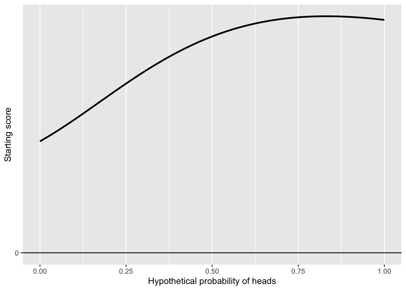
I don’t mean to suggest that the score function depicted in Figure fig-coin-flip-prior1 reflects any reality about coins. It is simply a function in the right format: It’s never negative. Most people, I suspect, would draw their personal score function with a peak near probability 0.5 and falling to near zero at the extremes of the interval. This is reasonable, since we all have prior experience with flipping coins showing heads about half the time. But if you had just walked into a gambling den, you might suspect that a cheating coin is being used.
Interpreted literally, the starting score function in Figure fig-coin-flip-prior1 reflects a belief the coin is somewhat biased toward heads. But this is not a big deal, since the lowest score is not dramatically different from the highest.
Sometimes, your honest opinion about hypothesis plausibility is, “I don’t have any opinion whatsoever.” This situation corresponds to a score function graph that is a horizontal line.
6.3.2 The likelihood
A “likelihood” is a conditional statement about the probability of each possible outcome. That is, the likelihood is a function whose input is a type of observation and whose output is a probability. In this coin-flipping example, the observations are “heads” or “tails.” These are the only two legitimate values for the input to the likelihood function.
Now let’s talk about “conditional statement.” This means that the statement applies only if a stated condition exists. Here’s an example: If it rains tomorrow, we’ll stay inside. The statement is, “We’ll stay inside.” The condition here is “it rains tomorrow.” Another example: If it is sunny tomorrow, we’ll go canoeing. Going canoeing is the statement, conditioned on it being sunny tomorrow. A conditional statement is not about what the condition is. In everyday terms, a conditional statement is a “what if.” Or, you might prefer to think about a conditional statement as a “plan”: If such-and-such a situation arises, we’ll say so-and-so.
In a likelihood, the condition is always a hypothesis. In the coin-flip, we have a large number of conditional statements, for instance x = 0.3 or x = 0.65 and so on. Each of these statments has its own likelihood function. For instance, the likelihood function corresponding to the hypotheses x = 0.3 has a form like, “The probability of observing heads is 0.48 and the probability of observing tails is 0.52.” You might notice that the clause about observing tails is redundant. If the probability of observing heads is 0.48 then it must be that the probability of observing tails is 1 - 0.48 = 0.52.
A likelihood function is not a matter of opinion. For each hypothesis under consideration, the likelihood is a calculation done on a hypothetical planet where the hypothesis is true. That is, we imagine that the hypothesis is true when doing the calculation. This is characteristic of “hypothetical reasoning,” the title of this tutorial.
I was wrong before when I used the numbers 0.48 and 1-0.48 - 0.52. That was an incorrect calculation for the likelihood function under the hypothesis that x = 0.3. You are going to do the correct calculation, for any given value of x. This won’t be difficult. But the calculation is so simple and obvious that it is hidden in plain sight. It’s along the lines of the question, “Who is buried in Grant’s Tomb.” Grant …. obviously!
Warm up exercise: Under the hypothesis that the probability of heads is 0.65, what is the probability of heads? You scratch your head. Didn’t we just say what the probability of heads is? Absolutely. Second question: under the stated hypothesis, what is the probability of tails? You’ll have to do a simple calculation to get the answer.
Now generalize to any of the competing hypotheses about the coin:
Under the hypothesis that that the probability of heads is p, what is the probability of heads?
You should be able to give the answer in one letter. Similarly, you should be able to answer the following question about the probability of tails, but it will take three characters:
Under the hypothesis that that the probability of heads is p, what is the probability of tails?
6.3.3 Implementing the likelihood function
Recall that a likelihood is the probability of observing a particular outcome, say H, according to the hypothesis under consideration. I have packaged up the likelihood calculation as an R function coin_likelihood(). The function takes the observation (either "H" or "T") as one input and the value of p as the other input. For instance, coin_likelihood("T", 0.75) will compute the likelihood of the observation T under the hypotheses that the probability of heads is 0.75.
Test out coin_likelihood() to make sure it does the right calculation for each of the possible observations and a given probability.
6.3.4 Calculating the posterior
Recall that the Bayesian step is to update the prior based on the new observation(s), and that, after we have the new observation(s), that is, in the post-observation world, the updated prior is called the posterior. The calculation is straightforward: multiply the prior by the likelihood of the new observation to get the posterior.
To implement the calculation, we need to express our personal prior as a function of x. Here’s my prior, which is merely an exception of my ignorance:
My_prior() says that any value of x is equally plausible to me, at least before (prior to) my collecting and processing data. (A stickler for detail might object: the above prior only makes sense if we restrict x to the domain 0 to 1. We’ll evade this objection by looking only in the domain 0 to 1.)
Here’s a plot of the prior:
Now, let’s imagine that we have observed a single T. Recall that p is the probability of H on a single flip. Consequently, the probability of T is (1-p).
Translating this to a likelihood function: the likelihood of observing T under the hypothesis “heads with probability p” is simply (1-p).
Having observed a new T, we can update the prior to produce the posterior. As always, the posterior is the likelihood of the new observation times the prior. Like the prior, the posterior is a function of p, so we’ll define it before plotting it.
Look carefully at the graph of the posterior after a single observation of T. The posterior for p = 1.00 (“heads, for sure”) is now zero. We can safely rule that out after even a single T observation. The most plausible hypothesis is p = 0.00 (“tails, for sure”). But other values of x are also somewhat plausible.
TASK: Modify the posterior() function in Active R chunk lst-posterior-T to represent what the situation would be if we had flipped twice, resulting first in a T then in an H.
6.4 Null hypothesis testing
If you have taken a statistics course before, you likely have heard of something called a “p-value” which is a result of a general procedure called “hypothesis testing.” So-called hypothesis-tests are heavily used as a guide to whether a scientific paper is “significant” enough for publication. Consequently, it’s important to know what a “hypothesis test” is …. and what it isn’t. For example, a “hypothesis test” is not a Bayesian computation to compare the plausibility of competing hypotheses. In fact, a “hypothesis test” involves only one hypothesis, not two or more competing hypotheses as with Bayes.
The single hypothesis involved in a “hypothesis test” is a statement about the world that can be expressed in a variety of ways in everyday English:
- Nothing of interest is going on in the system being studied.
- There’s nothing wrong with conventional wisdom about the system.
- There’s no relationship between two variables.
This “no”-filled hypothesis has a general name, the “Null hypothesis.
Before considering the logic and mathematics behind the p-value, we have to say something about the social and historical setting in which Null hypothesis testing came to play such a prominent role in science. Health and disease have always been important concerns. Ignaz Semmelweis (1818-1865) demonstrated that simple (now obvious) hygenic practices by physicians—washing hands between patients, cleaning instruments—could dramatically decrease maternal deaths in childbirth. His work was ignored and even disparaged by the medical community. Starting in the 1850s, Louis Pasteur introduced the “germ theory” of disease, a hypothesis that illnesses are caused by micro-organisms. First applications of germ theory were to the “pasteurization” of wine and milk, although it also explained Semmelweis’s findings about hygiene. Joseph Lister (1827-1912), a surgeon, hypothesized that post-surgical infection—a major cause of surgical mortality—was caused by germs. Lister proposed “anti-sepsis” as a way to reduce infection. This started an explosion of research work to identify particular micro-organisms that caused particular diseases.
Perhaps today it’s self-evident that merely spotting a specific micro-organism in diseased tissue is no adequate to demonstrate that the micro-organism causes the disease. A leading authority, Robert Koch (1843-1910) who won the Nobel Prize in 1902, proposed some general principles (called “postulates”) for justifying a claim that a particular micro-organism causes a particular disease.
The first postulate was:
The organism must always be present in every case of the disease, but not in healthy individuals.
There were three additional postulates, but the first will do for us here. Notice that it implies that in order to study disease, it is not sufficient to examine only people with the disease. You also have to examine healthy people and find a contrast. Today we use the term “control group” for the healthy people.
It’s easy today to think about Koch’s First Postulate in Bayesian terms. There are two hypotheses: the person is diseased or the person is healthy (the control). We look at the output of the likelihood function for the observation of the micro-organism. Translated (ahistorically) into Bayes, Koch’s postulate amounts to saying that the likelihood of observing the micro-organism under the diseased hypothesis should be 100%, while the likelihood under the healthy (control) hypothesis for that observation should be much smaller.
But the translation of Koch to Bayes did not happen. Instead, statistical pioneer Ronald Fisher (1890-1962), who in 1925 published the first how-to book on statistical calculations for science, Statistical Methods for Research Workers, decided to focus on the control group. The control group is well described by the Null hypothesis: nothing interesting is going on. At a minimum, Koch’s first postulate insists that the likelihood of observing the micro-organism, under the control hypothesis, is small.
Fisher was interested in situations where we look at an average (or such) to characterize the system. In hypothesis testing, we examine the likelihood, under the Null hypothesis, of the observed value (say, the average). Fisher developed formulas and tables for this likelihood under the Null. This is a purely mathematical matter because it’s easy to formulate the Null hypothesis in purely mathematical terms. The likelihood value that Fisher invented came eventually to be called the “p-value.”
Most statistics textbooks present Null hypothesis testing by following the historical pattern of development. This pedagogical approach has created well-known pathologies. Hardly anyone who uses Null hypothesis testing actually understands what it’s about. We are going to break with pedagogical tradition by presenting the p-value ahistorically, using a concept that was developed after the p-value was introduced. This concept is the confidence interval.
We will make another break with conventional statistics textbooks as well. Those books present several different “tests” that apply in various circumstances. But since we are using regression as our basic technique, all of the conventional tests amount to regression, for which we already know how to compute a confidence interval. (In the exercises, we will introduce the names for several common tests and show their equivalent using regression.)
Recall that the confidence interval on a model coefficient indicates the precision with which that coefficient has been measured. For instance, suppose we publish a coefficient as 3.2 \(\pm\) 1.5. Then someone comes along, claiming that 3.2 isn’t right. Instead, they claim, the true number is 4.5. Our only legitimate response is that 4.5 is a plausible value, consistent with our evidence. (Of course, the 4.5 claimant should give a confidence interval as well. If that includes our 3.2 then they have no good reason to challenge our claim.)
In terms of model coefficients, the Null hypothesis is almost always this simple statement: Under the Null, the coefficient is zero.
With a confidence interval in hand, it’s dead easy to carry out a hypothesis test. Simply check whether zero is inside the confidence interval. If it is, our data don’t lead us to reject the claim made by the Null. That is, we “fail to reject the Null.” But if the confidence interval excludes zero, we’re justified in “rejecting the Null.”
What about the p-value, where does that come from? FROM the confidence level used in constructing the confidence interval that just touches the value from the Null hypothesis. If we use a 95% confidence interval, the p-value is 5%. If we used a 99% confidence interval, the p-value would be 1%.
Scientists are people. People like to think they are important. For historical reasons that are unclear, the practice emerged of interpreting the p-value as measuring the importance of the reported work. This is nonsense, but people will be people. Pandering to such ideas, statistical formulas, tables, and software are arranged to find the highest confidence level for which the confidence interval touches zero. The p-value is reported as one minus this level. So you will often see p-values reported as p = 0.001 or smaller.
A much more informative approach is simply to publish the confidence interval. Readers can see for themselves whether zero is included. They also get a good idea about the effect size, which is the true measure of “how big an effect” has been detected.
For regression coefficients, to conduct a “hypothesis test,” simply check whether a coefficient of interest has a confidence interval that includes zero. Or, to get a p-value, find the confidence level at which the confidence interval just touches zero. To illustrate, consider the question of whether smoking is associated with mortality. We’ll model the Whickham data to test outcome ~ smoker and check the confidence interval on the smokerYes coefficient.
The smokerYes confidence interval, -6.3 to -1.3, does not contain zero, so we reject the Null hypothesis that smoking and mortality are unrelated. There is no real need to calculate a p-value, but if the journal editor insists, you can do it. Calculate the confidence interval at different confidence levels until the interval just barely touches zero.
For instance, the 99% confidence interval reaches closer toward zero, but doesn’t yet touch it.
If the confidence interval had touched zero, the p-value would be 1 - 0.99 = 0.01. At this point, the matter should rest and the researcher can appropriately claim \(p < 0.01\).
The software will display a p-value if you ask:
Let’s verify that the p-value on smokerYes leads to a confidence interval that just touches zero.
Many researchers like to use different language from “reject the Null hypothesis.” You will often hear, “The result is significant,” or, more honestly, “The result is statistical significant.” This statistical meaning of “significant” has little to do with the everyday meaning. Journalists especially attach great significance to “significant,” potentially misleading their readership. There is a movement in modern statistics to replace the archaic statistical term with one that avoids misleading. Instead of “significant,” use “discernible”.
As always, covariates can be very important, so the isolated p-value on smokerYes has little practical meaning. To illustrate, it’s well known that age is a predictor of mortality. And, at the time of the Whickham project, young women were more likely to smoke than older women, so age and mortality are confounded. Statistical adjustment gives some insight into the degree of confounding.
Notice that the p-value on smokerYes in Mod2 is 0.22, much larger than the 0.0027 from Mod1. P-values refer to a particular context, e.g. how big is the sample size, how the sample was collected, what covariates were used, whether there are interaction or nonlinear terms, and so on.
No answers yet collected