Activities E: Tutorial 5 – UATX Computing Tutorials: Data and Modeling

Activity E.1 Here is a simulation in which the variable X affects the variable Y.

You can see from the formula for Y that both X and C influence it to different extents. Here’s the simulation in causal diagram form:

Suppose we’re interested in the direct connection between X and Y, for instance, if X is the amount of an environmental toxin and Y is a measure of the immune response. C is some other factor, say poverty, that leads to a change in Y due to poor nutrition and also influences where the person lives.

Is C a confounder? Explain your reasoning.

We’re going to generate some data from the simulation and build a model Y ~ X to understand the effect of the toxin.

Active R chunk E.1

The coefficient on X is about 1/2. Looking at the simulation formula for Y, is this the right coefficient to capture the causal connection between X and Y. Explain your reasoning.

Because this is a simulation, we can easily conduct an experiment. What we will do is assign people to live in areas with different levels of the environmental toxin, then follow them over time to see what is the resulting effect of X on Y.

Recall that an experiment is an intervention that changes the causal network. The people will be alternately assigned to have environmental toxin levels of -1 and 1, as you can see in the very small sample

Active R chunk E.2

Here’s the simple model Y ~ X.

Active R chunk E.3

When data is collected from the experiment, does the model Y ~ X recover the correct causal connection (as seen in the simulation formula) between X and Y? (You can change the sample size to get a clearer view, if you like. Another nice feature of simulations!)

Change Active R chunk E.3 to add C as a covariate. Does this distort the model’s depiction of the causal connection between X and Y? Explain which coefficient you are looking at when forming your answer.

Finally, let’s return to the non-experimental situation as in Active R chunk E.1. This is called observational data because there is no intervention in the system . Add C as a covariate. Does this recover the correct causal link between X and Y? Explain which coefficient you are looking at when forming your answer.

Activity E.2 Consider this different causal network, Sim2, still involving X, C, and Y but connected in a somewhat different manner.

Active R chunk E.4

You can see from the formula for Y that both X and C influence it to different extents. Here’s the simulation in causal diagram form:

Explain what’s different between the geometry of Sim2 from that of Sim1 in Activity E.1.

Let’s start off, first thing, by setting up an experiment to see the causal link between X and Y.

Active R chunk E.5

Add commands to Active R chunk E.5 to take a sample of size 100, train the model Y ~ X, and look at the coefficients.

Is the coefficient on X consistent with the causal mechanism defined in Active R chunk E.4? (Feel free to increase the sample size if you need to in order to support your reasoning.)

Now include the covariate C in the model (that is, Y ~ X + C). Does this distort the apparent influence of X on Y? Try to explain as best you can what the covariate C is doing to the X coefficient.

Finally, let’s return to the observational data, as generated by Sim2. Take a sample from Sim2 and train three different models on it: Y ~ X, Y ~ C, and Y ~ X + C.

Does including C in the model help or hinder revealing the true causal connection between X and Y.

Activity E.3 To illustrate a RCT—randomized clinical trial— consider the “Prevención con Dieta Mediterránea” (PREDIMED), a 2003-2009 study of diet and risk of coronary heart disease involving about 7000 subjects. I use the word “subjects” rather than the more conventional “people” to emphasize that this was an experiment. Interventions were imposed by the researchers on the participants in the study. looking at the possible link between the Mediterranean.

In PREDIMED, subjects were randomly assigned to one of three groups: a control and two variations of a Mediterranean diet (“Nuts” and extra-virgin olive oil (VOO)). The point of random assignment is to avoid mixing the assigned group with covariates and lurking variables. The goal of random assignment is to achieve balance between the groups, ideally, that all groups have the same makeup of members. When a covariate is measured, the balance can be imposed by making sure that all levels of the covariate have equal numbers of subject assigned to each of the experimental groups. This is called blocking, that is, dividing the subjects into “blocks” with similar values for the covariates. But when lurking variables are involved, this is not possible; lurking variables are unknown. Thus, randomization is used to produce approximate balance even against the unknown variables.

We know that random assignment was used because the study authors told us so in their report. Ideally, a formal process is used involving computer random number generators rather than the haphazard choice of researchers which might be inadvertantly be influenced by patient characteristics. A sign (but not a guarantee) of blocking and random assignment is that the covariates are unrelated to the group assignment.

For simplicity of analysis, we’ll lump together the two Mediterranean diet groups into one and check if membership in control versus Mediterranean is unrelated to the covariates. Active R chunk E.6 does some basic wrangling to set up for later analysis:

Active R chunk E.6

Active R chunk E.7 looks at whether assignment to diet is related to model covariates. Ideally, it shouldn’t.

Active R chunk E.7

Ideally, the logistic regression coefficients for the covariates should be zero. They are mostly small, but some of the confidence intervals do not include zero. This is a sign that the randomization was not properly done. As an example of how important dialog is in scientific communication, see this abstract in The New England Journal of Medicine. Indeed, in the study summary, the researchers report:

In 2013, we reported the results for the primary end point in the Journal. We subsequently identified protocol deviations, including enrollment of household members without randomization, assignment to a study group without randomization of some participants at 1 of 11 study sites, and apparent inconsistent use of randomization tables at another site. We have withdrawn our previously published report and now report revised effect estimates based on analyses that do not rely exclusively on the assumption that all the participants were randomly assigned.

The retracted article is here. Note that “retracting” does not mean “removing from view.”

Tutorial 6 introduces p-values, which provides a concise summary of whether a confidence interval includes zero. To judge from the report above, what about the p-value indicates that the confidence interval doesn’t include zero?

Of course the primary point of the PREDIMED study is to examine the possible relationship between diet and coronary heart disease. Looking at whether the diet assigned is related to the covariates is just a check that the experimental protocol went as planned. The “protocol deviations” are certainly a “flaw” in the study. Critics love to point to such flaws; almost all studies have some flaw or another. But even a flawed study can give useful information. For instance, here, we can adjust for the covariates to attempt (mathematically) to strip their influence from the study. Active R chunk E.9 shows one such analysis.

Active R chunk E.8

The basic result from Active R chunk E.8 is that a Mediterranean diet (level = 1 in the diet variable) is associated with a … well, what. This is a linear model of a zero-one variable, so the coefficient can be interpreted as the absolute change in risk of an event. The coefficient is $- 0.011 \pm 0.010$ , that is, a 1% reduction in absolute risk.

Read through the entire report from Active R chunk E.8 and identify any covariates whose effect size is similar in magnitude—positive or negative—to that of diet. In addition, calculate the relative change in risk associated with each of those factors. For reference, note that the overall risk of an event, disregarding the explanatory variables, is about 4% for the people enrolled in the PREDIMED study.

We should be careful, however, about our choice of technique. The effect sizes of smokeNever and diet are pretty large compared to the baseline risk. The standard fix for this potential problem is to use logistic regressions. That’s easy enough.

Active R chunk E.9

Now the coefficient on diet is a whopping -0.28. But for mathematical reasons it takes care to interpret such coefficients. First, logistic regression looks at relative, not absolute change in risk. Second, the coefficients are denominated in strange-sounding units: the logarithm of the likelihood ratio. This is the ordinary logarithm from mathematics. You can convert it to a simple odds ratio with the exp() function. Active R chunk E.10 does this with the diet coefficient and the lower and upper bounds of the confidence interval.

Active R chunk E.10

It looks like the Mediterranean diet is associated with an odds ratio that reduces the odds of an event by about 24 percent (CI: 1 to 42 percent). Spiegelhalter (p. 34) briefly discusses when an odds ratio can be interpreted as an approximate risk ratio. Here, that approximation is pretty good.

Convert the coefficients for sexMale, diab, and smokeNever into confidence intervals on the odds ratio (which you might just as well interpret as relative risks). How do these compare in size to the odds ratio for diet?

A good topic for class discussion (in Tutorial 6) is why the author’s didn’t mention such factors in their results section. Another good topic for discussion is the relevance of an alternative endpoint generally preferred by epidemiologists: all cause mortality. See Figure 1 (A & B) in the article.

Statisticians often look at subgroups of the participants in the study. This may seem like common sense, but interferes with the simple interpretation of “statistical significance” via p-values as will be discussed in Tutorial 6.

In Tutorial 1 (Active R chunk A.9), as an example of graphics, we split up by sex the survival curves for the PREDIMED participants. There, it’s evident that survival for males is very different than for females, and also that the apparent effects of diet on survival are very different. So let’s look at the male “sub-group” to see what might appear.

Active R chunk E.11

Does the male-only subgroup suggest a different story than the whole-group results? Also, modify Active R chunk E.11 to conduct a female-only subgroup analysis and say whether those results suggest something different. Do you think it would have been appropriate to address this issue in the results reported? (Why they didn’t is another of those potential Tutorial 6 discussions.)

This has been a long, detailed examination of the PREDIMED study. But let’s take on one more issue: causality. Any recommendation that a Mediterranean diet is good for you centers on the idea that such a diet causes a reducted risk of coronary heart disease (or, better, all cause mortality). For many people, the use of experimental intervention is sufficient reason to justify causal conclusions. I don’t disagree with this except to note the uncertainty in the magnitude of the effect.

The key to the association between experiment and causal conclusions is that the experimenters assign the treatment (at random), and so any statistical connection between treatment and outcome must be causal (to the extent that it is not so small that it might be considered accidental, another Tutorial 6 topic). In experiments like this, however, the experimenter’s intent to treat (ITT in the diagram) is not the only thing that influences diet, the causal variable of interest. The subject’s level of compliance with the assigned diet is also a factor.

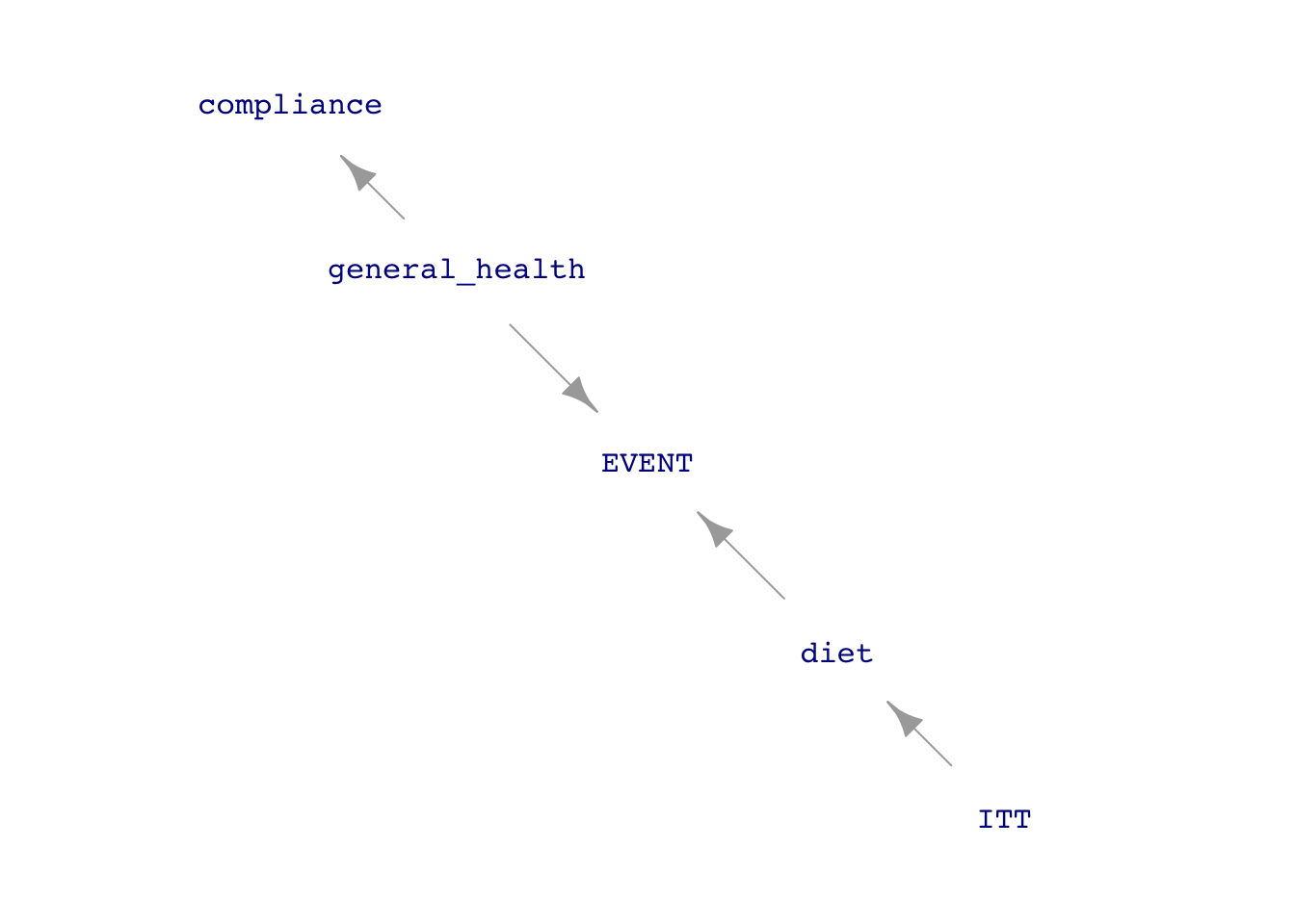
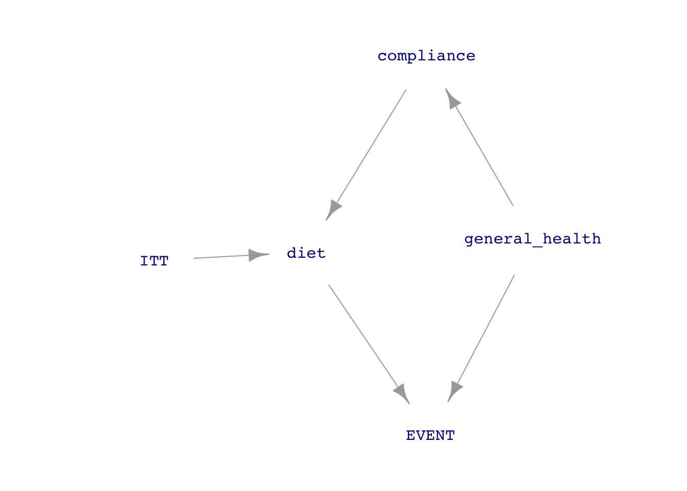
The diagram in Figure E.1 assumes perfect randomization of ITT. This appears as the absence of incoming arrows to ITT from the covariates. But even if this ideal had been achieved, the influence of compliance on diet creates a “back-door” pathway between diet and event. The experiment would have been pristine only if diet had no incoming arrows except that from ITT.

So, in Figure E.1(b), general health is a confounder between diet and EVENT. The causal interpretation of the analysis results presented above assumes that compliance is a trivial issue. But better if some measurement can be made of compliance so that it can be included as a covariate that will block the back-door pathway. The PREDIMED investigators included in their study a very rough indication of the ability to comply. They point out that it would be difficult to comply with a Mediterranean diet if the subject does not know what such a diet entails. They gave all the participants a questionnaire consisting of 14 questions about the Mediterranean diet. The p14 variable in Predimed gives the score from zero to fourteen. The investigators reconned that a score below ten means compliance was iffy.

Go back to Active R chunk E.9 or the male-only subgroup analysis Active R chunk E.11 and add p14 as a covariate. To what extent does this alter your interpretation of the results.

Activity E.4 IN DRAFT Example: Running time versus age. Cross-sectional versus longitudinal.

webR Code Links

R History Command Contents