Activities B: Tutorial 2 – UATX Computing Tutorials: Data and Modeling

Activity B.1

Which of the prediction intervals below is a match for the interval [20,30]?

What is the $\pm$ format that corresponds to the interval [3, 8]?

Which prediction interval is equivalent to 27 $\pm$ 6?

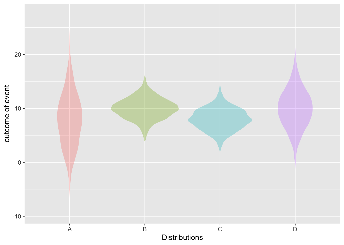
Recall that a prediction interval is merely shorthand for a distribution of probability over the possible outcomes of the event. Which of distributions in Figure B.1 corresponds to the interval 10 $\pm$ 4?

Figure B.1: Distributions for Activity B.1 (4).

Activity B.2 The Birdkeepers data frame has data from a study conducted in The Hague, Netherlands. Earlier work had discovered an association between birdkeeping and lung cancer. To follow up, the 1985 case-control study was conducted. The sample consisted of 49 people with lung cancer (the cases) and another 98 who were similar in terms of age but did not have lung cancer.

What was the prevalence of lung cancer in the case-control study population?

Case-control studies are designed specifically to over-represent the fraction of cases compared to the overall population. The prevalence in the study population was established by the design of the study rather than the risk of lung cancer in the broad population. Nonetheless, case-control studies can be very valuable at finding risk factors since they allow relative risks to be calculated.

We’re going to look at two possible risk factors for lung cancer: keeping a bird (BK) and having been a smoker for more than 20 years (long_smoker). Active R chunk B.1 defines the long_smoker variable.

Active R chunk B.1

First, let’s look at the bird-keeper risk factor on it’s own using the tabulation created in Active R chunk B.2.

Active R chunk B.2

What’s the risk ratio for lung cancer among birdkeepers (disregarding smoking status) compared to non-birdkeepers?

33 / 16

33 / (33 + 64) compared to 64 / (64 + 34)

33 / (33 + 34) compared to 16 / (16 + 64)

question id: 2-birdkeepers-2

A different tabulation let’s us look at long_smoker as a risk factor on its own. (Active R chunk B.3)

Active R chunk B.3

What’s the risk ratio for lung cancer among long smokers (disregarding birdkeeping status) compared to non-long-smokers?.

45 / 64

45 / (45 + 4) compared to 64 / (64 + 34)

45 / (45 + 64) compared to 4 / (4 + 34)

question id: 2-birdkeepers-3

Yet another calculation (Active R chunk B.4) is needed to take into consideration both of the risk factors at the same time.

Active R chunk B.4

What’s the risk ratio for lung cancer among people who have both risk factors compared to people who have neither risk factor?

30 / 22

30 / (30 + 22) compared to 1 / (1 + 22)

3 / (3 + 12) compared to 15 / (15 + 42)

question id: 2-birdkeepers-4

Refer back to the output about birdkeepers that doesn’t include long smoking as a risk factor. Think of a doctor asking “Do you keep a bird?” as a screening test for lung cancer. What is the sensitivity and specificity of such a test?

sensitivity 33 / (33 + 16); specificity 64 / (64 + 34)

sensitivity 64 / (64 + 34); specificity 33 / (33 + 16)

sensitivity 33 / (33 + 64); specificity 34 / (34 + 16)

question id: 2-birdkeepers-5

As mentioned in part 1 above, the prevalence in the case-control study group does not reflect the prevalence in the broad population. Let’s assume that the prevalence in the broad population is 2%. Using the sensitivity and specificity from question (5), for a person who keeps a bird (that is, has a positive test result), what is their personal risk of lung cancer? (Recall that the multiplier will be sensitivity / (1 - specificity).)

Activity B.3 The largest circulation magazine in the US is the AARP Bulletin, published by the American Association of Retired People. (Eligibility to join: age 50+). The December 2024 issue contained an article headlined, “Dollars and Dementia: An Early Warning System,” which reported a claim that credit-card delinquency is predictive a year or more in advance of a diagnosis of dementia. Delinquency rates one year before diagnosis were 50% higher than those six years before diagnosis.

To take a deeper look, one can read the medical journal research paper mentioned in the AARP article. For convenience, Table B.1 presents the facts in terms of the numbers in a population of 10,000 people:

Table B.1: In a population of 10,000 like those in the journal report, braking down the number who will be diagnosed with dementia and those who will have credit-card delinquency one year before any diagnosis.

	Dementia	OK
Delinquency	50	170
none	1450	8330

What’s the prevalence of dementia in the population?

What’s the accuracy of the dementia prediction using credit-card delinquency?

What’s the specificity of dementia prediction using credit-card delinquency?

What’s the sensitivity of dementia-sensitivity of dementia prediction using credit-card delinquency?

A random person selected from relevant population has a risk of developing dementia (in six years time) that is simply the prevalence. Suppose that one year before the end of the six-year period the person has a credit-card delinquency. This person’s risk has therefore gone up. The proportional increase in risk is sensitivity / (1 - specificity), which is here about 1.5.

Using all of the above, comment based on whether accuracy alone provides a good way to assess the utility of a screening test.

Activity B.4 It is often claimed that standardized college-entrance exam results are good predictors of success in college. Such claims usually don’t come with a definition of “good predictors.”

Figure B.2 shows the GPAs of about 4372 UT Austin graduates along with their entering standardized test scores, separately for STEM and non-STEM students.

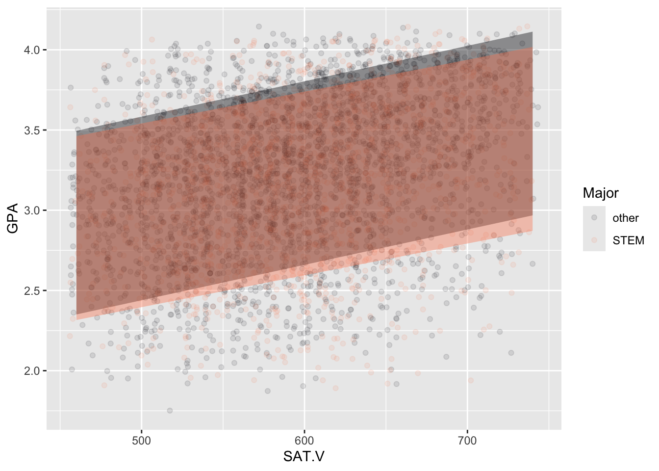
Based on the graph, comment on whether standardized test scores are a good predictor of GPA and whether the verbal or quantitative scores differ substantially in their predictive ability for STEM versus non-STEM students. Feel free to give arguments both pro and con.

Activity B.5 Figure B.3 shows two prediction models based on UTsat, the UT Austin data including whether a student will choose a STEM major.

UTsat |>
  point_plot(zero_one(Major, one = "STEM") ~ SAT.V, annot = "model",
             point_ink = 0.1, jitter = "x") |>
  gf_labs(y = "Probability of STEM major")
UTsat |>
  point_plot(zero_one(Major, one = "STEM") ~ SAT.Q, annot = "model",
             point_ink = 0.1, jitter = "x") |>
  gf_labs(y = "Probability of STEM major")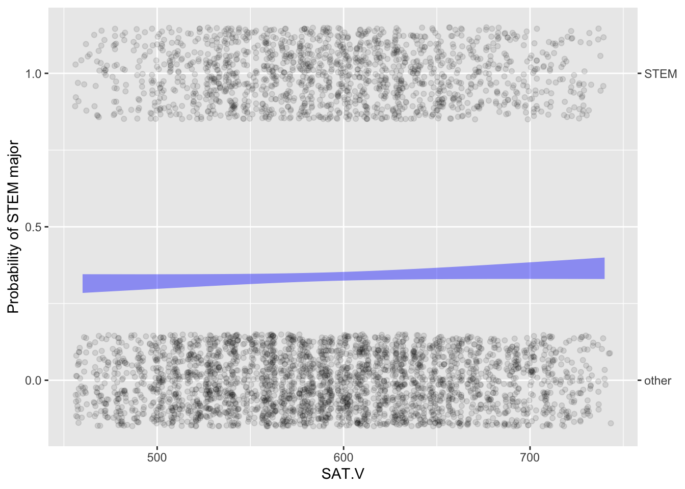

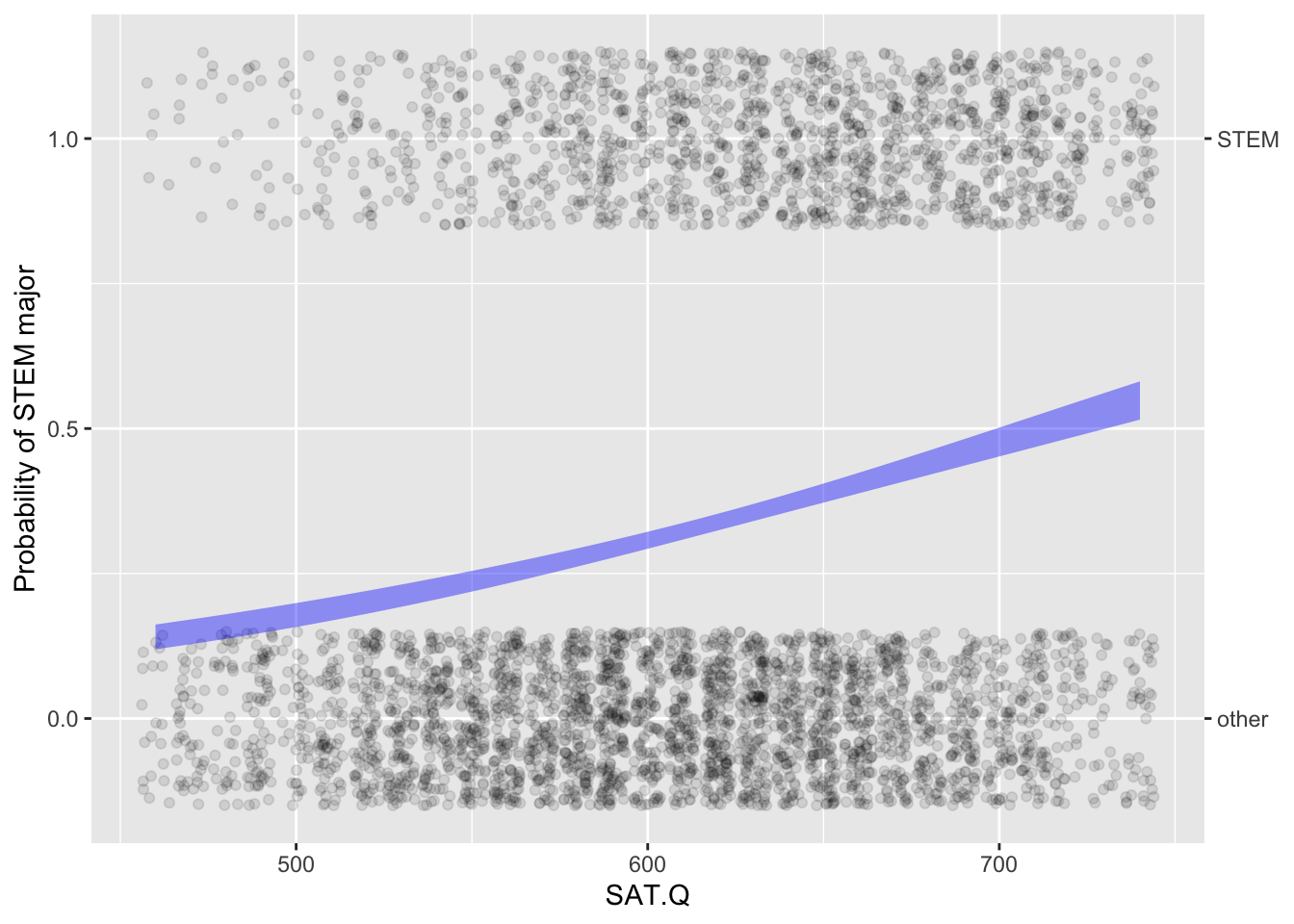
s What about the two models indicates that verbal SAT is useless for predicting majoring in STEM, but that quantitative SAT is somewhat predictive. At the same time, describe what the graph (b) would have looked like if quantitative SAT were a great predictor of majoring in STEM.

Activity B.6 Let’s consider the STEM prediction models from Activity B.5 in terms of two “screening test.” We will set a threshold for a “positive” test as an SAT score greater than 650. We are intentionally not telling you which performance table is for the verbal score and which for the quantitative score.

test_result	Major	count
neg	STEM	1199
neg	other	2325
pos	STEM	277
pos	other	571

test_result	Major	count
neg	STEM	867
neg	other	2193
pos	STEM	609
pos	other	703

Figure B.4: Performance of SAT score as STEM predictors.

Which of the tables in Figure B.4 is for the verbal score and which for the quantitative score?

Left table is for verbal

Right table is for verbal

There is no way to tell.

question id: stem-predict-1

Using the right-hand table, calculate the sensitivity of the test.

Using the right-hand table, calculate the specificity of the test.

Activity B.7 In the tutorial, using the Whickham data frame, we computed a Brier score of 0.112 for the survival predictions from the model outcome01 ~ age + smoker.

Active R chunk B.5

The first command in Active R chunk B.5, that is, the one starting with Whickham <- Whickham |> ..., does some setting up for the modeling. Explain exactly what is being done by that first command.

Why is model_eval() used in the third command in Active R chunk B.5?

To put the score 0.112 in context, we need to compare the score to that from a “Null” model with no explanatory variables. In the tilde expression in Active R chunk B.6, the 1 is simply a placeholder meaning “no explanatory variables.”

Active R chunk B.6

Insert the appropriate command in the last line of Active R chunk B.6 to calculate the Brier score on the Null model

The “skill” of the survival model looks at the reduction in residual variance produced by the explanatory variables as a proportion of the null-model residual variance.

Calculate the “skill” of the Survive_model predictions using the Brier scores from Survive_model and the Null model. The formula is:

$Skill \equiv \frac{Null_Brier - Prediction_brier}{Null_Brier}$

What is the skill?

What aspect of the model specification outcome01 ~ 1 is consistent with the “null” in the term “Null model?

Activity B.8 Activity A.9 looked at the survival curves from the PREDIMED study. Figure B.5 shows the survival curves for the different diets (but not broken down by sex).

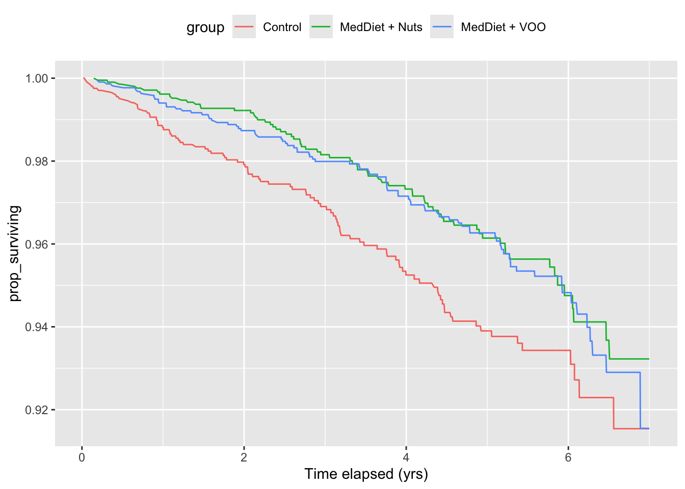
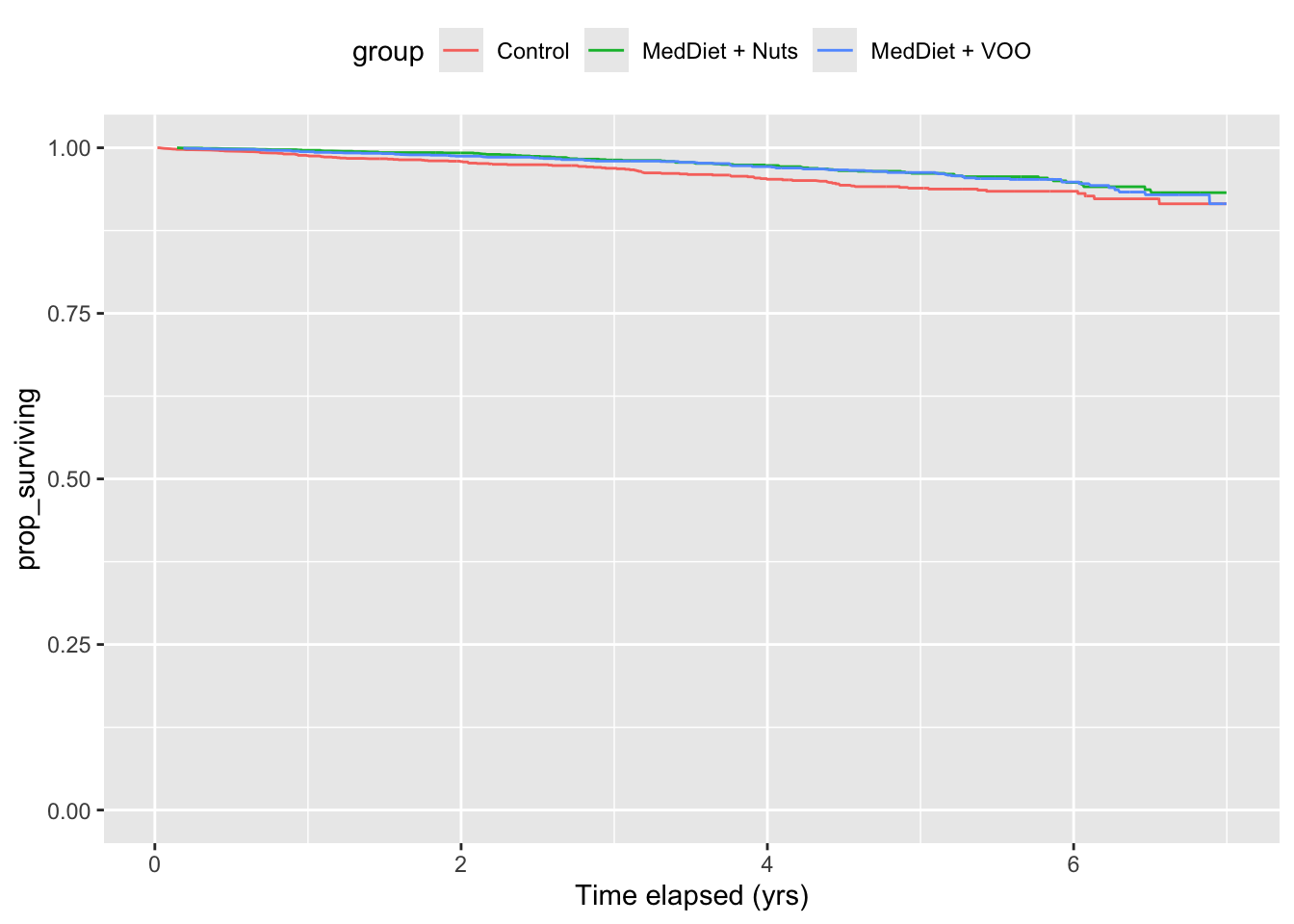
The two graphs show the same three survival curves, but look vary different. Which style, (a) or (b), emphasizes relative risk and which emphasizes absolute risk? Comment as well on whether relative or absolute risk would be more useful to a general audience of people interested in making a decision about switching to a Mediterranean diet.

webR Code Links

R History Command Contents