Activities F: Tutorial 6
Remember to hand in your work …
At any point, you can submit your answers by collecting them and uploading them to the class site.
No answers yet collected
If the answers that have been loaded automatically are not yours, press this button before starting your work:
Activity F.1
During an imagined debate at UT Austin, it was claimed that there are “hugely significant” differences between grade distributions in different schools. A summary of the model GPA ~ School was put forward as supporting evidence.
- What about the ANOVA summary is or is not consistent with the use of “hugely significant?”
Another debater points to an R2 summary of the same model, saying that the ANOVA report is misleading and that, in reality, there is practically no difference in GPAs between schools.
- Explain what in the R2 summmary supports the claim of “practically no difference in GPAs.” At the same time, explain whether the R2 report is inconsistent with the ANOVA summary.
Activity F.2 In Section 3.5.3, we used ANOVA to compare two models of Galton’s heights. Now that we know about Null hypothesis testing and p-values, we will look at four models.
Interpret the ANOVA summary format from Active R chunk F.1 as sequentially comparing models. We start with the Null model. Having no explanatory variables, none of the variation in the response variable can be accounted for. Then move to the second model, which has mother as the explanatory variables. Can mother explain some of the variation in height? The p-value for the corresponding line of the ANOVA summary looks at the likelihood that a purely random variable unrelated to height (say, the last number in the home address of the child’s grandmother’s uncle) could account for as much variation in height as does mother. That’s a bit of a complicated explanation, so let’s be informal and shorten it: The p-value tells whether mother has anything to say about height.
The next line of the ANOVA summary looks at adding father as an explanatory variable. Again, the p-value in that line tells us whether father has something to contribute to explaining height beyond what mother can explain.
The last line of the ANOVA summary compares an even “larger” model, ~ mother + father + nkids, to the previous model. Using the informal explanation, the p-value tells us whether nkids has something to add to the explanation of height.
- True or False:
Motheraccounts forheightto a significant extent.
6-nkids-meaning-a
- True or False:
Fatheraccounts for something significant beyond whatmotherhas already accounted for.
6-nkids-meaning-b
- True or False:
nkidsalso adds a significant explanation ofheight.
6-nkids-meaning-c
Now let’s consider some common, harmful, and avoidable mis-interpretations of the ANOVA summary.
“Significant” means something in everyday English and something else in statistics. In statistics it means that the p-value was small, where “small” is generally taken to be p < 0.05.
A smaller p-value tells something about how strong the relationship is. For instance, the p-value for
fatheris about one-million times smaller than the p-value formother. Does this mean that fathers have a more important influence than mothers on their children’s height? Not at all! To look at the relative strength of influence, look at the relative effect sizes, as in Active R chunk F.2.
Although the father coefficient is larger than that for mother, the two confidence intervals overlap strongly. Galton’s data do not support a hypothesis that fathers have a greater influence than mothers.
Since the p-value on nkids is p < 0.01, nkids also has something to say about a child’s height. Looking at the effect size of nkids tells us that larger nkids corresponds to a shorter child (by one-tenth of an inch per addition family member). So far, so good. But then the mis-interpreters go too far, all while sounding reasonable. “We speculate that children in larger families are slightly shorter because there is more competition for nutrition and greater exposure to contagious illness.”
Forming speculative hypotheses is an important activity in science, and there’s nothing wrong with using an ANOVA summary to spark the imagination. But at least look at your data with an eye to refuting the hypothesis before foisting it on your readership.
Here, there is a well-known variable strongly associated with height that was not included in the models: sex.
- Go back to Active R chunk F.1 and add
sexas a covariate in all of the models. Look at the resulting ANOVA summary and explain what this suggests aboutnkidsinfluencing height.
Why did including sex as a covariate increase the p-value on nkids. Whenever this sort of thing happens, it’s because the two values (sex and nkids here) are related to one another. So, is nkids related to the fraction of females? We’ll turn to this in Activity F.4.
Activity F.3 Traditional statistics courses include a half-dozen or so named tests, each of which has it’s own formula and procedure to turn the result of the formula into a p-value. It’s helpful to know the names of these tests so that you can perform them using dataframe |> model_train(...) |> conf_interval()
- one-sample p-test produces a confidence interval on a proportion. To conduct a hypothesis test, check whether the Null hypothesis value is in the confidence interval.
Example: Is the proportion of males and females in the Galton data consistent with a 50-50 split between the sexes?
Galton |>
  model_train(I(sex == "F") ~ 1, family = "linear") |>
  conf_interval()
# A tibble: 1 × 4
term .lwr .coef .upr
<chr> <dbl> <dbl> <dbl>
1 (Intercept) 0.449 0.482 0.515- one-sample t test produces a confidence interval for the mean of a quantitative response variable. The hypothesis test merely checks whether the Null hypothesis value is inside the confidence interval.
Question: Is the mean height of the full-grown children in Galton consistent with a hypothesized 66 inches?
True or false: We can reject the Null hypothesis
one-sample-t
- two-sample p test looks at the difference between two proportions. For instance, defining “tall” to be 69 inches or higher, is the fraction women who are tall different from the faction of men who are tall?
First, we need to do some wrangling to calculate who is tall, which we will encode with 0:
Galton |>
  mutate(tall = (height >= 69)) |>
  model_train(tall ~ sex, family = "linear") |>
  conf_interval()
# A tibble: 2 × 4
term .lwr .coef .upr
<chr> <dbl> <dbl> <dbl>
1 (Intercept) -0.00307 0.0323 0.0677
2 sexM 0.506 0.555 0.604 The Null hypothesis in our question is that the difference between the sexes of the fraction of tall people is zero. There are two terms reported. Which is the right one to look at the difference between the sexes?
two-sample-p
- two-sample t test looks at the difference between two means. For instance, mean height for women different from the mean height for men. The Null hypothesis value is zero.
Galton |>
  mutate(tall = (height >= 69)) |>
  model_train(height ~ sex, family = "linear") |>
  conf_interval()
# A tibble: 2 × 4
term .lwr .coef .upr
<chr> <dbl> <dbl> <dbl>
1 (Intercept) 63.9 64.1 64.3
2 sexM 4.79 5.12 5.45Which term’s confidence interval should you look at, and should you reject or fail to reject the Null hypothesis?
two-sample-t
- t-test for regression checks whether a slope from a regression model is consistent with a Null hypothesis of zero. For instance, do taller women tend to marry taller men?
Galton |>
  model_train(mother ~ father, family = "linear") |>
  conf_interval()
# A tibble: 2 × 4
term .lwr .coef .upr
<chr> <dbl> <dbl> <dbl>
1 (Intercept) 55.1 59.3 63.6
2 father 0.00773 0.0688 0.130Which term’s confidence interval should you look at, and should you reject or fail to reject the Null hypothesis?
regression-t
one-way chi-squared test considers whether the counts of a categorical variable are consistent with some hypothesized proportion. The chi-squared test is one of the historically earliest statistical tests, and it doesn’t provide either an effect size nor a confidence interval.
two-way chi-squared test looks at whether the levels of two categorical variables are related. The Null hypothesis is that they are not. In QR2, we use logistic regression instead. This has both advantages and disadvantages. Logistic regression is restricted to a binary response variable, which chi-squared can handle multi-level categorical variables. On the other hand, logistic regression can include covariates. Logistic regression is very widely used in clinical studies, chi-squared not so much.
Example, is the probability of being a girl related to the height of the mother? The Null hypothesis is that it is not.
Galton |>
  mutate(girl = zero_one(sex, one = "F")) |>
  model_train(girl ~ mother) |>
  conf_interval()
# A tibble: 2 × 4
term .lwr .coef .upr
<chr> <dbl> <dbl> <dbl>
1 (Intercept) -5.72 -2.06 1.59
2 mother -0.0258 0.0310 0.0881
mother-determines-sex
- one-way ANOVA looks at the differences in means of a quantitative variable between two or more groups. For instance, does bill length depend on which of the three islands in
Penguinsthat a penguin lives on. The Null hypothesis is that it does not.
Penguins |>
  model_train(bill_length ~ island) |>
  anova_summary()
# A tibble: 2 × 6
term df sumsq meansq statistic p.value
<chr> <int> <dbl> <dbl> <dbl> <dbl>
1 island 2 1417. 709. 27.5 9.21e-12
2 Residuals 330 8512. 25.8 NA NA True or false: We can reject the Null hypothesis
one-way-anova
- two-way ANOVA looks at the means of a quantitative variable with respect to two categorical explanatory variables. The question is whether the means are related to both the explanatory variables. This is a matter of looking at the interaction term between the two explanatory variables. In the tilde expression, take note of the use of
*to specify that an interaction term be used.
Example: Is the difference in bill length by island different for the two sexes? (Mathematically, this is exactly equivalent to a question framed by reversing the two explanatory variables: “Is the difference in bill length by sex different between the three islands?”) The Null hypothesis is “no,” that is, island and sex do not jointly influence the bill length.
Penguins |>
  model_train(bill_length ~ island * sex) |>
  anova_summary()
# A tibble: 4 × 6
term df sumsq meansq statistic p.value
<chr> <int> <dbl> <dbl> <dbl> <dbl>
1 island 2 1417. 709. 31.5 3.17e-13
2 sex 1 1142. 1142. 50.7 6.79e-12
3 island:sex 2 6.17 3.09 0.137 8.72e- 1
4 Residuals 327 7363. 22.5 NA NA What’s potentially confusing here is that this ANOVA summary can be used for three different hypothesis tests:
- Does the mean bill length depend on
island? (Answer: YES) - Does the mean bill length depend on
sex? (ANSWER: YES)
And the question that “two-way ANOVA” is specifically focussed on:
- Is there an interaction between
islandandsexin accounting forbill_length?
Looking at the row of the ANOVA summary that corresponds to the interaction, can you reject the Null hypothesis that the interaction component is no stronger than random noise?
two-way-anova
Activity F.8 Researchers conducting a careful study have many decisions to make about the details of data collection and analysis. If the p-value is to be taken at face value, the researchers have to fix the decisions before looking at the data. For instance, diligent researchers sometimes register their plans with a third party who can confirm that the eventually published results reflect the plans.
Understandably, many researchers would rather avoid restrictive planning. For instance, they may want to figure out the analysis procedure as they go along, but otherwise stick to accepted statistical procedures.
Let’s look at an example of what can happen when restrictive planning is avoided. I’ll use the Predimed data, but do not mean to suggest any problem with their published results. I just want to show how things can go wrong.
The Predimed data frame has records from a 2003-2009 study of about 7000 people looking at the possible link between the Mediterranean diet and risk of coronary heart disease. The study name was named “Prevención con Dieta Mediterránea,” thus the name “Predimed.” The work was published in a prestigious journal, The New England Journal of Medicine.
As part of the research process, the researchers made careful definitions before the study started. For instance, they decided how many subjects to (try to) enroll, what the study interventions would be, and what the measured outcome would be: “cardiac events” such as infarction, stroke, and so on. They also fixed a target follow-up duration. As always, since humans are involved, things don’t always go exactly to plan, for instance, studies often enroll somewhat fewer subjects than planned or lose track of people during follow-up. In the PREDIMED study, in fact, after initial publication, it was discovered that at some of the clinics involved improper randomization was used to assign subjects to diet treatments. The journal article listed above withdrew the first publication (without denying or hiding its existence) and re-analyzed the data without the problematic clinics.
Here, in brief, is the analysis planned and eventually conducted by the PREDIMED researchers: the risk of cardiac events as a function of the diet group. There are several relevant covariates that were included: sex, age, smoking status, body-mass index at enrollment, diabetes, family history of coronary heart disease, and a measure of non-compliance (p14) with the assigned diet, among others. But we will simplify and use just age, sex, and diet group as explanatory variables. Active R chunk F.3 does the calculations:
Positive coefficients indicate a positive association with risk of a cardiac event. We’re not directly interested in the age and sex covariates. (That’s what makes them covariates!) There were three diet groups: a control, and two somewhat different Mediterranean diets. The “Nuts” variation shows negative coefficient, meaning that it is protective against a cardiac event. The p-value makes it a publishable finding: p < 0.02. The “VOO” (extra-virgin olive oil) variation also has a negative coefficient, but the p-value is too high: p < 0.19.
Let’s look now at some things the researchers could have done to make their results seem more conclusive.
- Both the “Nuts” and “VOO” diets are Mediterranean. Do we really have to consider them separately? Here’s what happens if we do a little wrangling to combine them.
With this change, there is less ambiguity about the effects of the Mediterranean diet. The p-value is now p < 0.05. A simpler story.
- Subjects often do not comply with the assigned diet. To look at the compliance issue, the researchers gave the subjects a questionnaire about the components of the Mediterranean diet. They reasoned that if the score on the questionnaire was low, the subjects couldn’t have complied even if they wanted to. The questionnaire score, stored as
p14, runs from 0 to 14. The researchers figured that a score less than 10 means the subject could not comply well. For the subjects in the MedDiet groups, only about 40% got a score of 10 or higher.
But if there wasn’t strong compliance, any effect of the diet would be washed out. So how about if we use p14 >= 10 as the explanatory variable instead of the actual diet?
Much more exciting results: the coefficient on compliedyes is more negative than before and the p-value is much below the 0.05 threshold. Indeed, p < 0.0005!
You might wonder: why would a survey score taken by all subjects at the start of the experiment be predictive? The survey score doesn’t tell which diet the subjects were assigned to. And you might remember the matter of “intent to treat” described by Spiegelhalter.
- How about if we use
dietas the explanatory variable and merely adjust forp14. Try it and report what you found.
- The
cardiac_endpointresponse variable tells only if the subject had a cardiac event at some point during the study follow-up period. Might it not be better to include a more subtle measure of risk that includes how long it was until the event. We can reason that events that occurred very late indicate somewhat lowered risk. For mathematical consistency, we will assign ascoreinversely proportion to the time to the event, and zero if there was no event at all. In mathematical terms, “no event” means it took an infinitely long time to the event.
- Explain what using the risk score has accomplished in terms of detecting the salutory effects of the Mediterranean diet. At the same time, check whether using the
p14survey result is predictive of risk.
In the actual study, the researchers were careful to use “intent to treat.” Here’s the summary from the research paper:
A primary end-point event occurred in 288 participants; there were 96 events in the group assigned to a Mediterranean diet with extra-virgin olive oil (3.8%), 83 in the group assigned to a Mediterranean diet with nuts (3.4%), and 109 in the control group (4.4%). In the intention-to-treat analysis including all the participants and adjusting for baseline characteristics and propensity scores, the hazard ratio was 0.69 (95% confidence interval [CI], 0.53 to 0.91) for a Mediterranean diet with extra-virgin olive oil and 0.72 (95% CI, 0.54 to 0.95) for a Mediterranean diet with nuts, as compared with the control diet. Results were similar after the omission of 1588 participants whose study-group assignments were known or suspected to have departed from the protocol.
Activity F.4 In Activity F.2 we speculated that the relationship between nkids and the fraction of females might explain why children in larger families appear to be slightly shorter than children in smaller families. Of course, there might be other explanations, too, such as smaller families having better access to food, etc.
We don’t have any data about food, so there’s no way directly to test explanations involving food, interesting though that might be.
But we do have data on sex, so let’s figure out what we can say using that. First approach: Look at the fraction of girls in families of different sizes. Active R chunk F.7 does that.
Galton |>
  summarize(probF = mean(sex == "F"), .by = nkids) |>
  arrange(nkids)
nkids probF
1 1 0.4687500
2 2 0.4500000
3 3 0.4696970
4 4 0.4137931
5 5 0.4357143
6 6 0.5000000
7 7 0.5446429
8 8 0.4765625
9 9 0.5079365
10 10 0.6000000
11 11 0.5312500
12 15 0.5333333- Explain what pattern, if any, is revealed by the wrangling statements. If you like, build a model
probF ~ nkidsto do a hypothesis test on the pattern.
The speculation that bigger families have shorter children can be usefully re-stated by splitting it up:
- Bigger families have shorter daughters, and/or
- Bigger families have shorter sons.
Let’s look at the (possible) relationship between nkids and height separately for males and females.
Galton |> filter(sex == "F") |>
  model_train(height ~ mother + father + nkids) |>
  conf_interval(show_p = TRUE)
# A tibble: 4 × 5
term .lwr .coef .upr p.value
<chr> <dbl> <dbl> <dbl> <dbl>
1 (Intercept) 9.49 16.8 24.2 8.39e- 6
2 mother 0.224 0.307 0.390 1.59e-12
3 father 0.325 0.399 0.472 8.26e-24
4 nkids -0.0797 -0.00861 0.0625 8.12e- 1Galton |> filter(sex == "M") |>
model_train(height ~ mother + father + nkids) |>
conf_interval(show_p = TRUE)# A tibble: 4 × 5
term .lwr .coef .upr p.value
<chr> <dbl> <dbl> <dbl> <dbl>
1 (Intercept) 12.2 20.4 28.6 1.24e- 6
2 mother 0.244 0.334 0.424 1.42e-12
3 father 0.312 0.403 0.495 9.84e-17
4 nkids -0.158 -0.0786 0.000946 5.28e- 2- Interpret the result from Active R chunk F.8, explaining what it does (or does not) tell you about the relationship between
nkidsandheight.
F.1 In-class activities
Activity F.5 We’re going to play “Paper-rock-scissors.” One of the players will be H, the other T. Whoever wins determines the outcome of the game. Your task is to figure out how many games must be played to be practically sure that the outcome is fair. Or, if one of the players is weak, how many games must be played to see a clear sign of this weakness.
Play many games. After each, add the result of that game to the string of H and T used in coin_likelihood() and plot the posterior score function. (Note the quotation marks around the HTH… string. These tell the R system not to interpret the letters as the name of some function or variable.)
What did you discover?
Activity F.6 Let’s talk a little about Bayesian priors, that is, the starting score you use. There are two limiting situations:
- You have very strong opinions about the matter.
- You don’t have any strong opinion.
In case (2), it’s reasonable to use a constant prior; one that’s the same for all hypotheses. You can implement this as in Active R chunk F.9, or, more simply, just leave the * prior(p) out of the calculation.
In case (1), the temptation is to express your opinion in the calculations. We’re going to play with this, giving you a simulator to express “stong” opinions in the rock-paper-scissors game you used in Activity F.5. The mathematics behind the simulator isn’t important to us here, but we can use it even without a complete understanding of it.
The mathematical “beta function” is often used to represent various functions that are non-negative over the interval zero to one. It has two parameters, which you can set to give the shape of function that you want. Both parameters must be non-negative. Here’s a sandbox to experiment with:
prior <- function(p) dbeta(p, 0.5, 2.0)
slice_plot(prior(p) ~ p, domain(p = 0:1))
Be aware that there is nothing special about beta functions in this application. They are simply a convenient way to describe a shape to the computer.
Play around with the beta shape parameters to identify four appropriate pairs for these four different situations:
- You are almost sure that the game is strongly biased toward T.
- You are almost sure that the game is strongly biased toward H.
- You are almost sure that the game is balanced between T and H.
- You have no idea whether or not the game is biased.
Now return to Activity F.5. Implement each of the four priors (i) through (iv) using the observations made in your series of rock-paper-scissors games. Can you discern the impact of the priors in the face of the actual observations?
Activity F.7 At casinos, all the games are carefully arranged so that the casino, called the “house,” is somewhat favored to win. In each game, the gambler places a bet. If the gambler wins, the house pays him back his bet plus an extra amount. If the gambler loses, the bet goes to the house. It’s helpful to think about the percentage of the total amount gambled that the house “takes.” For slot machines, the take is about 5%. If casinos had a coin-flip game where heads is a win for the gambler, to have a take of 5% the probability of heads needs to be 47.5%.
To explain this, imagine that in one evening 10,000 plays are made. On average, the house will win 52.5% of the time, being paid $1 each play. For the 47.5% of plays where the gambler wins, the house is paid -$1, that is, pays the gamber $1. That is, out of the 10,000 plays for the evning, there are 5250 where the house wins and 4750 where the house loses. Total winnings: $5250 - $4750 = $500, that is, 5% of the $10,000 put into the game by customers.
A likelihood function summarizes what the observed data has to say about the situation. (In contrast, the prior conveys what you have to say about the situation before the data were collected.) There are two sets of data involved in this problem. One is the casino’s observations, say, of 10,000 plays. The other data is from the customer’s perspective, say, of 100 plays. Let’s examine whether these two perspectives lead to the same conclusions even when the customer’s data is entirely consistent with the casino’s data.
Figure F.1(a) shows the likelihood function for an observed 4750 wins by customers out of 10,000 plays. This is the casino’s point of view. But a single customer might play only 100 games. Suppose the customer has 47 wins out of 100. The likelihood function corresponding to this data is shown in (b).
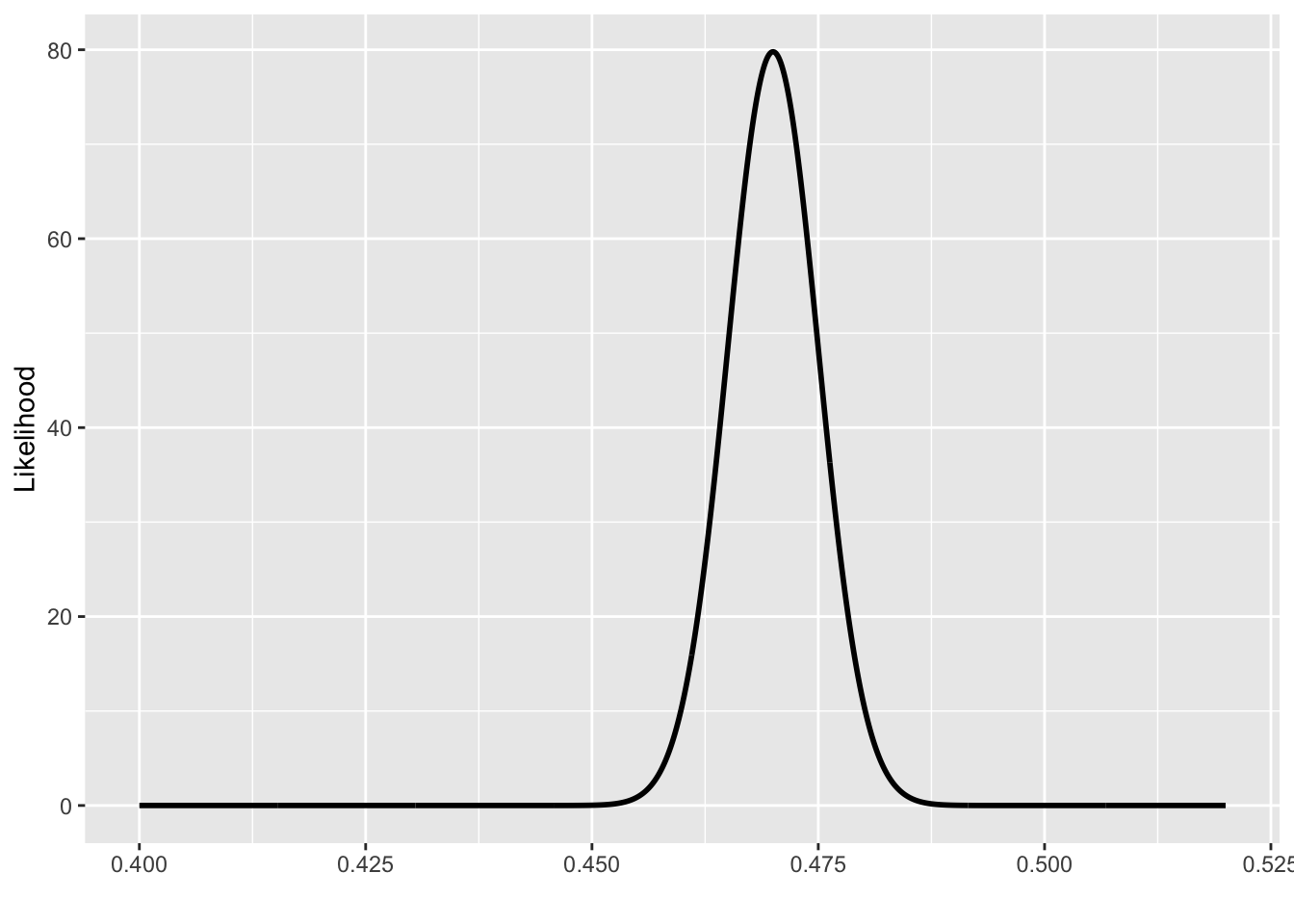
Casino's point of view = “10,000 plays with 4750 heads”)
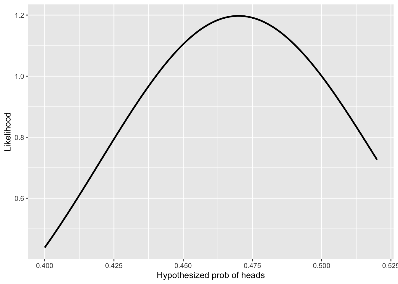
Gambler's point of view = “100 plays with 47 heads”)
The casino has accountants who keep track of each night’s earnings. Similarly, the state has a gambling commission to keep an eye on the casinos. One purpose for this is to prevent cheating by corrupt employees or tax-dodging by the casinos.
- Referring to the likelihood function in Figure F.1(a), will the casino and state gambling commission have any reason to think that the rigged coin has been replaced by a fair coin? Explain what about the likelihood function points to your computing.
Similarly, the customer wants to keep an eye out for cheating by the casino. The customer has less data: 47 wins out of 100 plays.
- Referring to the likelihood function in Figure F.1(b), does the customer have any good reason from his results to doubt that the coin is fair?
No answers yet collected