5 Accuracy, confounding and adjustment
computing
R
Remember to hand in your work …
At any point, you can submit your answers by collecting them and uploading them to the class site.
No answers yet collected
If the answers that have been loaded automatically are not yours, press this button before starting your work:
5.1 Objectives
- Distinguish properly between “accuracy” and “precision” in the statistical sense.
- Precision is measured with confidence intervals.
- Accuracy can not be measured from data.
- When causality is an issue, accuracy is important.
- Be able to interpret and work with “causal influence diagrams” (also known as DAGs: “directed acyclic graphs”) which is a way to encode a hypothesis about networks of causal connections.
- Understand how confounding can arise in a causal network and lead to inaccurate models.
- Use covariates and adjustment properly to correspond to any given hypothesis about causal influences.
5.2 Introduction
Many statistics books include a diagram like Figure fig-bullseye to illustrate the distinction between accuracy and precision.

The archery diagram is often effective as an explanation. That’s why so many books use it. But everyday usage of the words “precision” and “accuracy” overlaps so much that it is hard to keep track, without the labels in the diagram of which is which. Good synonyms for “precision” are “reliability” or “repeatability”: you get about the same result every time you try. Confidence intervals are a statistical method to describe precision. But there’s an important caveat: confidence intervals tell you nothing about accuracy.
Traditional statistics books have two things to say about accuracy, neither of which comes directly from data. Instead, it’s the **meta-data* that gives a clue about accuracy: how the data were collected.
To give accurate results, the data should be a census or sampled at random. This requires that you have access to every potential specimen, not a situation that arises in practice very often. It’s hard to achieve a random sample: many statistics books have long sections on sources of sampling bias. The problem is so hard that even the US Census does not produce a census in the statistical sense: a complete enumeration of every member of the population.
When a causal relationship between two (or more) variables is at issue, data should be collected by experimental intervention. In such an intervention, the experimenter assigns values of the explanatory variable. For the results to provide accuracy, such assignment should be made at random.
Randomly in this sampling and assignment context does not mean haphazardly. It takes deliberate and considerable effort to plausibly implement randomness. The practical difficulties of achieving randomness in a political poll have rendered the high-stakes polls largely useless.
In this tutorial, we will be mainly concerned with making accurate statements about causal chains. These are particularly important when it comes to making decisions about a potential action. Accuracy lets us know what the action is likely to accomplish, be it taking a pill or implementing programs to distribute anti-malarial mosquito netting among people at risk.
An experiment with random assignment is an excellent approach to such accuracy … if it can be done. There are many settings where experiment is not an option. Reasons include ethics (randomly assign people to smoke to see if smoking causes cancer), non-compliance (you assign people to take a drug, but will they comply), pollution (you assign other people to a placebo, but they are skeptical and seek treatment elsewhere), but there are many others. For instance, is parole from prison effective at reducing recidivism? You can’t really assign parole at random both for political reasons (“soft on crime”) and the law.
The difficulties of experiment and random assignment are such that Spiegelhalter devotes an entire section (pp. 114-119) to the question, “Can we ever conclude causation from observational data?” But better to ask, “Is there a set of criteria for helping us judge when causal conclusion are reasonable?” In fact, Spiegelhalter starts out his section by referring to such a set of criteria, promulgated by Austin Bradford Hill, that are widely accepted in science. (Most statistics teachers have never heard of these, even though Hill was president of the Royal Statistical Society.)
Bradford Hill’s nine criteria are presented in the Proceedings of the Royal Society of Medicine. His essay is a model of readability. Only one of the nine criteria relates to experiment. It’s worth quoting in full because it doesn’t even point to the practice of random assignment:
Criterion 8: Experiment: Occasionally it is possible to appeal to experimental, or semi-experimental, evidence. For example, because of an observed association some preventive action is taken. Does it in fact prevent? The dust in the workshop is reduced, lubricating oils are changed, persons stop smoking cigarettes. Is the frequency of the associated events affected? Here the strongest support for the causation hypothesis may be revealed.
Since there are many situations where causal hypotheses are central to a proposed action, it’s important to have statistical methods that can aid us in making responsible claims about causation.
5.3 Causal hypotheses
To review:
- Accuracy is about the extent to which conclusions match the actual, real-world situation.
- Statistics is about drawing conclusions from data. These conclusions inevitably involve choices made by the modeler and the limitations of his or her environment. Conclusion are therefore, to some extent, subjective.
How can we assess accuracy in the face of the subjectivity injected into the conclusion-making process? We will do this by introducing a framework for reasoning about accuracy. A realizable goal for this framework is that it help in drawing useful conclusions. Consequently, we will turn to a framework that is in broad use by people who have to make decisions about actions in the real world and which seem to have guided actions that produce beneficial outcomes.
This framework involves a causal hypothesis. We will see more about hypothetical thinking generally in Tutorial 6, but a bit of intuition will suffice here.
A causal hypothesis is a statement about what variables are relevant to our objective and how those variables are connected causally. Imagine, for instance, that our objective is to understand whether a particular medicine (pill) helps in improving patients’ outcomes, such as five-year survival. We also hypothesize that each patient has a general health status that we can measure in some way, e.g. blood chemistry or daily activity, or whatever.
To be more specific, we might imagine a particular set of causal connections, in which both a patient’s values of pill and health influence outcome, as in Figure fig-pill-health(a).
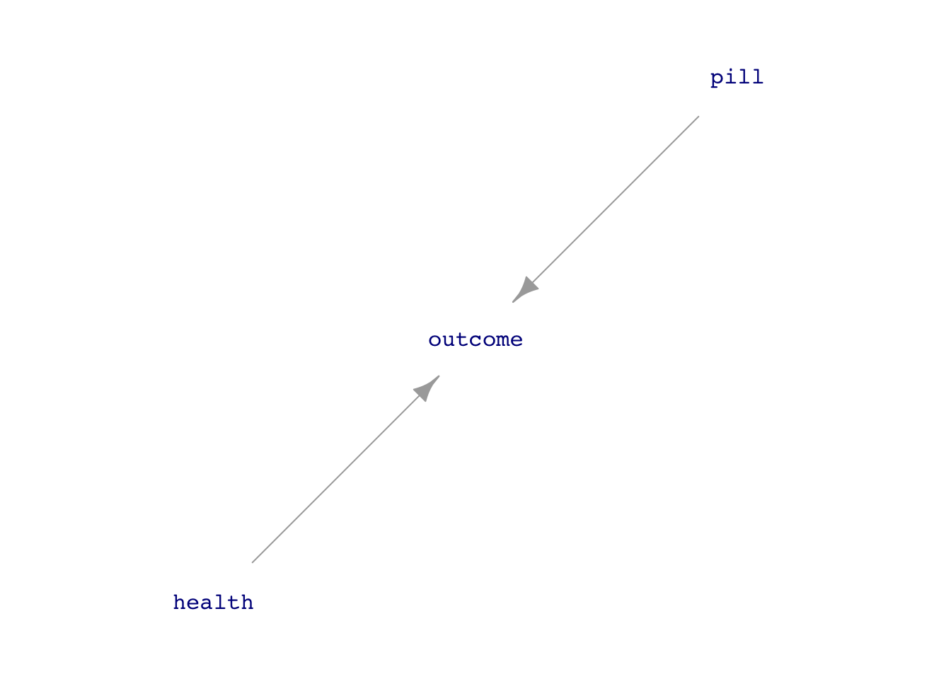
All that is being claimed in Figure fig-pill-health(a) is that both whether the patient takes the pill and general health contribute to the patient’s outcome. The diagram, called a “directed acyclic graph,” or DAG for short, doesn’t make any specific claim about whether the pill helps, hurts, or is irrelevant.
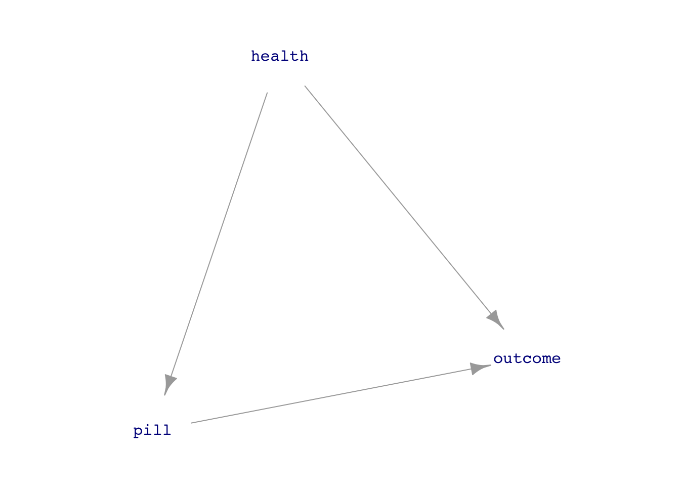
Figure fig-pill-health(b) is a different causal hypothesis to describe the situation. It claims the same contribution of pill and health to the outcome but adds in a twist: the patient’s health influences whether they take the pill. Perhaps some healthy people deny that they need medicine and don’t take it. Or, conversely, perhaps sick people can’t tolerate the medicine and avoid taking it. (Or both!)
We are going to encode each causal hypotheses with such an influence diagrams. The only restrictions on the notation are these:
- The arrows go only one way; there are no two-headed arrows. This is the “directed” in DAG.
- There are no loops of causation where a chain of arrows points back to where it started from. This is the “acyclic” in DAG.
Simply stating a hypothesis does not make it “true.” It is merely a hypothesis.
Now, returning to “accuracy” of conclusions drawn from data. Our framework is that accuracy is always conditioned on a hypothesis. For example, the model specification outcome ~ pill will provide accurate estimates under the hypothesis in Figure fig-pill-health(a) but not necessarily under the hypothesis in Figure fig-pill-health(b).
5.4 Confounding
The causal hypothesis in Figure fig-pill-health(b) is an example of confounding. The statistical meaning of “confounding” is, happily, well aligned with the everyday meaning. As defined by the Oxford Languages dictionary, “confounding” is:
- cause surprise or confusion in (someone), especially by acting against their expectations.
- mix up (something) with something else so that the individual elements become difficult to distinguish.
The confounding variable in Figure fig-pill-health(b) is health, which has both a direct influence on the outcome and mixes up with pill. The debate about pill might go like this:
Rudolph: I’ve just analyzed the data from our study using
outcome ~ pill. The data shows that taking a pill is leading to better outcomes.
Angie: I disagree. I think that what we’re seeing in the data is the result of confounding by health. Healthy people are more likely to take the pill, and healthy people have better outcomes.
The disagreement can be amicably resolved here by comparing the results from two models:
outcome ~ pilloutcome ~ pill + healthwhich adjusts forhealth.
Disagreements about more complicated causal hypotheses sometimes can be resolved by including covariates in a model, sometimes can be resolved by excluding potential covariates, and sometimes can’t be resolved at all. Due to the work of Judea Pearl (mentioned in Spiegelhalter), there is a way to analyze a DAG to determine which, if any, covariates should be included to produce an accurate estimate of the relationship of interest.
Of course, if health had not been measured—that is, if health were a lurking variable—no resolution between the simple hypotheses in Figure fig-pill-health would have been possible.
5.5 Experiment
Understandably, many people reject the idea that there is a role for subjectivity in proper scientific work. Consequently, they disfavor the idea that accuracy is conditioned on causal hypotheses. Instead, they propose sorting out causality by intervening in the real-world system, creating what is called a RCT, read either as “randomized control study” or (equivalently) as “randomized clinical study.” In other words, an experiment.
Historically, the idea of using randomization was controversial, but it is now accepted as the gold standard for experimental studies. In the activities, we will confirm that RCTs can create accurate results, but we will interpret this in terms of causal hypotheses: the experimental works in the world to impose structure on whatever the causal network might otherwise be.
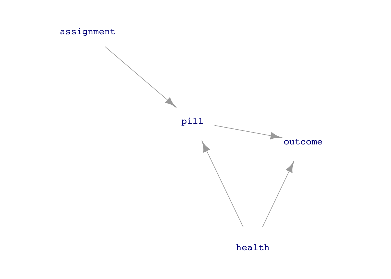
Figure fig-experiment-dags shows two DAGs relevant to interpreting an experiment about the pill-health-outcome network. The key idea is for the experimenter to take control of the pill variable by assignment of its value.
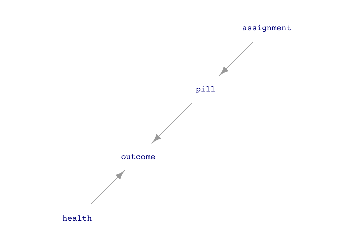
assignment. The overall system can still be described by causal influence diagrams.
As you’ll see, the simple model outcome ~ pill gives accurate results for Figure fig-experiment-dags(a).
But ideal experiments are not always possible. The model outcome ~ pill + health will give accurate results for both of the causal hypotheses in Figure fig-experiment-dags. What to do when confounders like health are not measured or measurable? A surprising result is that outcome ~ assignment, called “intent-to-treat analysis” is helpful. Econometricians prefer a more sophisticated kind of analysis, called “instrumental variables.” Here, assignment is the instrument. Leading proponents of instrumental variables, Joshua D. Angrist and Guido W. Imbens, were awarded the 2021 Nobel Prize in economics for their work, but understanding it requires technical, mathematical skills that not everyone possesses. For those with a particular interest in economics, this Nobel Committee report gives a somewhat accessible account.
5.6 Software
In the activities, we’ll use datasim_make() to construct simulations, dag_draw() to display the corresponding DAGs, and take_sample() to generate data from the simulation so that we can confirm the rules about whether including covariates in a model can produce accurate estimates.
No answers yet collected