Chapter 4 Solving

4.1 Functions vs equations

Much of the content of high-school algebra involves “solving.” In the typical situation, you have an equation, say \[ 3 x + 2 = y\] and you are asked to “solve” the equation for $x$. This involves rearranging the symbols of the equation in the familiar ways, e.g., moving the $2$ to the right hand side and dividing by the $3$. These steps, originally termed “balancing” and “reduction” are summarized in the original meaning of the arabic word “al-jabr” (that is, used by Muhammad ibn Musa al-Khowarizmi (c. 780-850) in his “Compendious Book on Calculation by Completion and Balancing”. This is where our word “algebra” originates.

High school students are also taught a variety of ad hoc techniques for solving in particular situations. For example, the quadratic equation $a x^2 + b x + c = 0$ can be solved by application of the procedures of “factoring,” or “completing the square,” or use of the quadratic formula: \[x = \frac{-b \pm \sqrt{b^2 - 4ac}}{2a} .\] Parts of this formula can be traced back to at least the year 628 in the writings of Brahmagupta, an Indian mathematician, but the complete formula seems to date from Simon Stevin in Europe in 1594, and was published by René Descartes in 1637.

For some problems, students are taught named operations that involve the inverse of functions. For instance, to solve $\sin(x) = y$, one simply writes down $x = \arcsin(y)$ without any detail on how to find $\arcsin$ beyond “use a calculator” or, in the old days, “use a table from a book.”

4.1.1 From Equations to Zeros of Functions

With all of this emphasis on procedures such as factoring and moving symbols back and forth around an $=$ sign, students naturally ask, “How do I solve equations in R?”

The answer is surprisingly simple, but to understand it, you need to have a different perspective on what it means to “solve” and where the concept of “equation” comes in.

The general form of the problem that is typically used in numerical calculations on the computer is that the equation to be solved is really a function to be inverted. That is, for numerical computation, the problem should be stated like this:

You have a function $f(x)$. You happen to know the form of the function $f$ and the value of the output $y$ for some unknown input value $x$. Your problem is to find the input $x$ given the function $f$ and the output value $y$.

One way to solve such problems is to find the inverse of $f$. This is often written $f^{\ -1}$ (which many students understandably but mistakenly take to mean $1/f(x)$). But finding the inverse of $f$ can be very difficult and is overkill. Instead, the problem can be handled by finding the zeros of $f$.

If you can plot out the function $f(x)$ for a range of $x$, you can easily find the zeros. Just find where the $x$ where the function crosses the $y$-axis. This works for any function, even ones that are so complicated that there aren’t algebraic procedures for finding a solution.
To illustrate, consider the function $g()$

g <- makeFun(sin(x^2)*cos(sqrt(x^4 + 3 )-x^2) - x + 1 ~ x)
slice_plot(g(x) ~ x, domain(x = -3:3)) %>%
  gf_hline(yintercept  = 0, color = "red")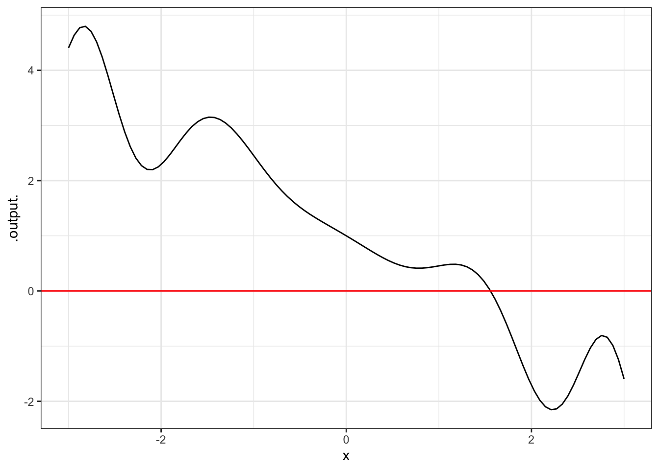

You can see easily enough that the function crosses the $y$ axis somewhere between $x=1$ and $x=2$. You can get more detail by zooming in around the approximate solution:

slice_plot(g(x) ~ x, domain(x=1:2)) %>%
  gf_hline(yintercept = 0, color = "red")

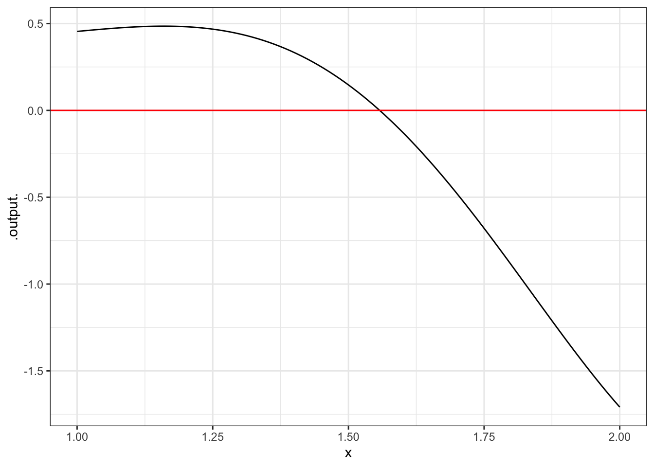The crossing is at roughly $x \approx 1.6$. You could, of course, zoom in further to get a better approximation. Or, you can let the software do this for you:

findZeros(g(x) ~ x, xlim = range(1, 2))

##        x
## 1 1.5576

The argument xlim is used to state where to look for a solution. (Due to a software bug, it’s always called xlim even if you use a variable other than x in your expression.)

You need only have a rough idea of where the solution is. For example:

findZeros(g(x) ~ x, xlim = range(-1000,  1000))

##        x
## 1 1.5576

findZeros() will only look inside the interval you give it. It will do a more precise job if you can state the interval in a narrow way.

4.1.2 Multiple Solutions

The findZeros( ) function will try to find multiple solutions if they exist. For instance, the equation $\sin x = 0.35$ has an infinite number of solutions. Here are some of them:

findZeros( sin(x) - 0.35 ~ x, xlim=range(-20,20) )

##           x
## 1  -12.2088
## 2   -9.7823
## 3   -5.9256
## 4   -3.4991
## 5    0.3576
## 6    2.7840
## 7    6.6407
## 8    9.0672
## 9   12.9239
## 10  15.3504

Note that the equation $\sin x = 0.35$ was turned into a function sin(3) - 0.35.

4.1.3 Setting up a Problem

As the name suggests, findZeros( ) finds the zeros of functions. You can set up any solution problem in this form. For example, suppose you want to solve $4 + e^{k t} = 2^{b t}$ for $b$, letting the parameter $k$ be $k=0.00035$. You may, of course, remember how to do this problem using logarithms. But here’s the set up for findZeros( ):

g <- makeFun(4 + exp(k*t) - 2^(b*t) ~ b, k=0.00035, t=1)
findZeros( g(b) ~ b , xlim=range(-1000, 1000) )

##       b
## 1 2.322

Note that numerical values for both $b$ and $t$ were given. But in the original problem, there was no statement of the value of $t$. This shows one of the advantages of the algebraic techniques. If you solve the problem algebraically, you’ll quickly see that the $t$ cancels out on both sides of the equation. The numerical findZeros( ) function doesn’t know the rules of algebra, so it can’t figure this out. Of course, you can try other values of $t$ to make sure that $t$ doesn’t matter.

findZeros( g(b, t=2) ~ b, xlim=range(-1000,1000) )

##        b
## 1 1.1611

4.1.4 Exercises

4.1.4.1 Exercise 1

Solve the equation $\sin(\cos(x^2) - x) - x = 0.5$ for $x$. {0.0000,0.1328,0.2098,0.3654,0.4217}

ANSWER:

findZeros( sin(cos(x^2) - x) -x - 0.5 ~ x, xlim=range(-10,10))

##        x
## 1 0.2098

4.1.4.2 Exercise 2

Find any zeros of the function $3 e^{- t/5} \sin(\frac{2\pi}{2} t)$ that are between $t=1$ and $t=10$.

There aren’t any zeros in that interval.}
There aren’t any zeros at all!}
$ 2, 4, 6, 8$}
$ 1, 3, 5, 7, 9$}
{$1, 2, 3, 4, 5, 6, 7, 8, 9$}

ANSWER:

findZeros( 3*exp(-t/5)*sin(pi*t) ~ t, xlim=range(1,10))

##    t
## 1  0
## 2  1
## 3  2
## 4  3
## 5  4
## 6  5
## 7  6
## 8  7
## 9  8
## 10 9

4.1.4.3 Exercise 3

Use findZeros() to find the zeros of each of these polynomials:

$3 x^2 +7 x - 10$

Where are the zeros? a. $x=-3.33$ or $1$ b. $x=3.33$ or $1$ c. $x=-3.33$ or $-1$ d. $x=3.33$ or $-1$ e. No zeros

ANSWER:

findZeros( 3*x^2 + 7*x - 10 ~ x, xlim=range(-100,100))

##         x
## 1 -3.3334
## 2  1.0000

$4 x^2 -2 x + 20$

Where are the zeros? a. $x=-3.33$ or $1$} b. $x=3.33$ or $1$} c. $x=-3.33$ or $-1$} d. $x=3.33$ or $-1$} e. No zeros

$2 x^3 - 4x^2 - 3x - 10$

Which one of these is a zero? {-1.0627,0,1.5432,1.8011,2.1223,3.0363,none}

ANSWER:

findZeros(2*x^3 - 4*x^2 - 3*x - 10 ~ x, xlim=c(-10,10))

##        x
## 1 3.0363

$7x^4 - 2 x^3 - 4x^2 - 3x - 10$

Which one of these is a zero? {-1.0627,0,1.5432,1.8011,2.1223,3.0363,none}

ANSWER:

findZeros( 7*x^4 -2*x^3 - 4*x^2 - 3*x - 10 ~ x, xlim=c(-10,10))

##         x
## 1 -1.0628
## 2  1.4123

$6 x^5 -7x^4 - 2 x^3 - 4x^2 - 3x - 10$

Which one of these is a zero? {-1.0627,0,1.5432,1.8012,2.1223,3.0363,none}

ANSWER:

findZeros( 6*x^5-7*x^4 -2*x^3 - 4*x^2 - 3*x - 10 ~ x, xlim=c(-10,10))

##        x
## 1 1.8012