Chapter 7 Derivatives and differentiation
As with all computations, the operator for taking derivatives, D() takes inputs and produces an output. In fact, compared to many operators, D() is quite simple: it takes just one input.
- Input: an expression using the
~notation. Examples:x^2~xorsin(x^2)~xory*cos(x)~y
On the left of the ~ is a mathematical expression, written in correct R notation, that will evaluate to a number when numerical values are available for all of the quantities referenced. On the right of the ~ is the variable with respect to which the derivative is to be taken. By no means need this be called x or y; any valid variable name is allowed.
The output produced by D() is a function. The function will list as arguments all of the variables contained in the input expression. You can then evaluate the output function for particular numerical values of the arguments in order to find the value of the derivative function.
For example:
## [1] 2## [1] 77.1 Formulas and Numerical Difference
When the expression is relatively simple and composed of basic mathematical functions, D() will often return a function that contains a mathematical formula. For instance, in the above example
## function (x)
## 2 * x
## <bytecode: 0x7fb3973d7e20>
For other input expressions, D() will return a function that is based on a numerical approximation to the derivative — you can’t ``see" the derivative, but it is there inside the numerical approximation method:
## function (x)
## numerical.first.partial(.function, .wrt, .hstep, match.call())
## <environment: 0x7fb3b1ea8bf0>
7.2 Symbolic Parameters
You can include symbolic parameters in an expression being input to D(), for example:
The parameters, in this case A, P, and C, will be turned into arguments to the s2() function. Note that pi is understood to be the number \(\pi\), not a parameter.
## function (t, A, P, C)
## A * (cos(2 * pi * t/P) * (2 * pi/P))
The s2() function thus created will work like any other mathematical function, but you will need to specify numerical values for the symbolic parameters when you evaluate the function:
## function (t, A, P, C)
## A * (cos(2 * pi * t/P) * (2 * pi/P))## [1] -0.3883222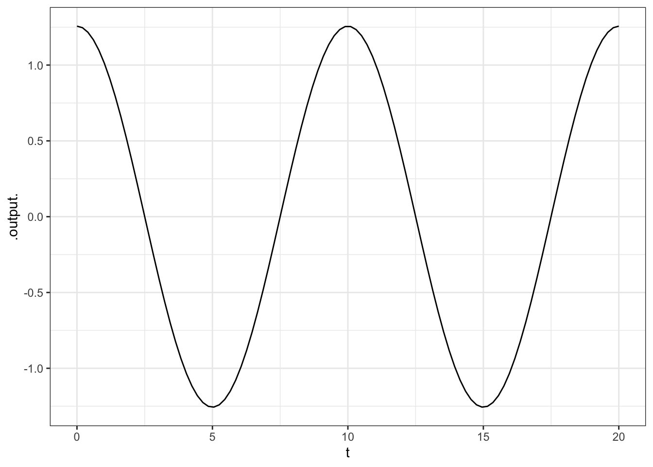
7.3 Partial Derivatives
The derivatives computed by D( ) are partial derivatives. That is, they are derivatives where the variable on the right-hand side of ~ is changed and all other variables are held constant.
7.3.1 Second derivatives
A second derivative is merely the derivative of a derivative. You can use the D( ) operator twice to find a second derivative, like this.
To save typing, particularly when there is more than one variable involved in the expression, you can put multiple variables to the right of the ~ sign, as in this second derivative with respect to \(x\):
This form for second and higher-order derivatives also delivers more accurate computations.
7.3.2 Exercises
7.3.2.1 Exercise 1
Using D(), find the derivative of 3 * x ^ 2 - 2*x + 4 ~ x.
What is the value of the derivative at \(x=0\)? {-6,-4,-3,-2,0,2,3,4,6}
What does a graph of the derivative function look like? a. A negative sloping line #. A positive sloping line #. An upward-facing parabola #. A downward-facing parabola
7.3.2.2 Exercise 2
Using D(), find the derivative of 5 * exp(0.2 * x) ~ x.
What is the value of the derivative at \(x=0\)? {-5,-2,-1,0,1,2,5}.
Plot out both the original exponential expression and its derivative. How are they related to each other?
- They are the same function
- Same exponential shape, but different initial values
- The derivative has a faster exponential increase
- The derivative shows an exponential decay
7.3.2.3 Exercise 3
Use D() to find the derivative of \(e^{-x^2}\) with respect to \(x\) (that is, exp(-(x^2) ~ x). Graph the derivative from \(x=-2\) to 2. What does the graph look like?
- A bell-shaped mountain
- Exponential growth
- A positive wave followed by a negative wave
- A negative wave followed by a positive wave
7.3.2.4 Exercise 4
What will be the value of this derivative?
- 0 everywhere
- 1 everywhere
- A positive sloping line
- A negative sloping line
7.3.2.5 Exercise 5
Use D() to find the 3rd derivative of cos(2 * t). If you do this by using the ~t&t&t notation, you will be able to read off a formula for the 3rd derivative.
- What is it?
- \(\sin(t)\)
- \(\sin(2 t)\)
- \(4 \sin(2 t)\)
- \(8 \sin(2 t)\)
- \(16 \sin(2 t)\)
- What’s the 4th derivative?
- \(\cos(t)\)
- \(\cos(2 t)\)
- \(4 \cos(2 t)\)
- \(8 \cos(2 t)\)
- \(16 \cos(2 t)\)
7.3.2.6 Exercise 6
Compute and graph the 4th derivative of cos(2 * t ^ 2) ~ t from \(t=0\) to 5.
- What does the graph look like?
- A constant
- A cosine whose period decreases as \(t\) gets bigger
- A cosine whose amplitude increases and whose period decreases as \(t\) gets bigger
- A cosine whose amplitude decreases and whose period increases as \(t\) gets bigger
- For
cos(2 * t ^ 2) ~ tthe fourth derivate is a complicated-looking expression made up of simpler expressions. What functions appear in the complicated expression?- sin and cos functions
- cos, squaring, multiplication and addition
- cos, sin, squaring, multiplication and addition
- log, cos, sin, squaring, multiplication and addition
7.3.2.7 Exercise 7
Consider the expression x * sin(y) involving variables \(x\) and \(y\). Use D( ) to compute several derivative functions: the partial with respect to \(x\), the partial with respect to \(y\), the second partial derivative with respect to \(x\), the second partial derivative with respect to \(y\), and these two mixed partials:
Pick several \((x,y)\) pairs and evaluate each of the derivative functions at them. Use the results to answer the following:
- The partials with respect to \(x\) and to \(y\) are identical. T or F
- The second partials with respect to \(x\) and to \(y\) are identical. T or F
- The two mixed partials are identical. That is, it doesn’t matter whether you differentiate first with respect to \(x\) and then \(y\), or vice versa. T or F