Chapter 9 Dynamics
A basic strategy in calculus is to divide a challenging problem into easier bits, and then put together the bits to find the overall solution. Thus, areas are reduced to integrating heights. Volumes come from integrating areas. Differential equations provide an important and compelling setting for illustrating the calculus strategy, while also providing insight into modeling approaches and a better understanding of real-world phenomena. A differential equation relates the instantaneous “state” of a system to the instantaneous change of state.
9.1 Solving differential equations
“Solving” a differential equation amounts to finding the value of the state as a function of independent variables. In an “ordinary differential equations,” there is only one independent variable, typically called time. In a “partial differential equation,” there are two or more dependent variables, for example, time and space.
The integrateODE() function solves an ordinary differential equation starting at a given initial condition of the state.
To illustrate, here is the differential equation corresponding to logistic growth:
\[\frac{dx}{dt} = r x (1-x/K).\]
There is a state \(x\). The equation describes how the change in state over time, \(dx/dt\) is a function of the state. The typical application of the logistic equation is to limited population growth; for \(x < K\) the population grows while for \(x > K\) the population decays. The state \(x = K\) is a “stable equilibrium.” It’s an equilbrium because, when \(x = K\), the change of state is nil: \(dx/dt = 0\). It’s stable, because a slight change in state will incur growth or decay that brings the system back to the equilibrium. The state \(x = 0\) is an unstable equilibrium.
The algebraic solution to this equation is a staple of calculus books.4 It is
\[x(t) = \frac{K x(0)}{x(0) + (K − x(0)e^{−rt})}\]
The solution gives the state as a function of time, \(x(t)\), whereas the differential equation gives the change in state as a function of the state itself. The initial value of the state (the “initial condition”) is \(x(0)\), that is, x at time zero.
The logistic equation is much beloved because of this algebraic solution. Equations that are very closely related in their phenomenology, do not have analytic solutions.
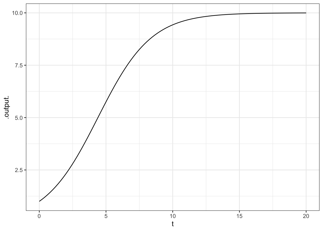
The integrateODE() function takes the differential equation as an input, together with the initial value of the state. Numerical values for all parameters must be specified, as they would in any case to draw a graph of the solution. In addition, must specify the range of time for which you want the function \(x(t)\). For example, here’s the solution for time running from 0 to 20.
The object that is created by integrateODE() is a function of time. Or, rather, it is a set of solutions, one for each of the state variables. In the logistic equation, there is only one state variable \(x\). Finding the value of \(x\) at time \(t\) means evaluating the solution function at that \(t\). Here are the values at \(t = 0,1,...,5\).
## [1] 1.000000 1.548281 2.319693 3.324279 4.508531 5.751209Often, you will plot out the solution against time:
9.2 Systems of differential equations
Differential equation systems with more than one state variable can be handled as well. To illustrate, here is the SIR model of the spread of epidemics, in which the state is the number of susceptibles \(S\) and the number of infectives \(I\) in the population. Susceptibles become infective by meeting an infective, infectives recover and leave the system. There is one equation for the change in \(S\) and a corresponding equation for the change in \(I\). The initial \(I = 1\), corresponding to the start of the epidemic.
epi <- integrateODE(dS ~ -a * S * I,
                    dI ~ a * S * I - b * I,
                    a = 0.0026, b = 0.5, S=762, I = 1,
                    tdur = 20)
This system of two differential equations is solved to produce two functions, \(S(t)\) and \(I(t)\).
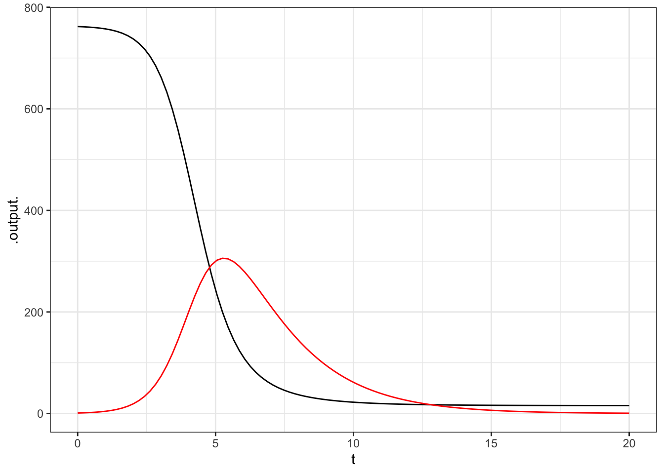
In the solution, you can see the epidemic grow to a peak near \(t = 5\). At this point, the number of susceptibles has fallen so sharply that the number of infectives starts to fall as well. In the end, almost every susceptible has been infected.
9.2.1 Example: Diving from the high board
Consider a diver as she jumps off the 5-meter high board and plunges into the water. In particular, suppose you want to understand the forces at work. To do so, you construct a dynamical model with state variables \(v\) (velocity) and \(x\) (position). As you may remember from physics, a falling object will accelerate downward at an acceleration of 9.8 meters per sec2. We’ll specify that the initial jump on the board is upward at a velocity of 1 meter per sec.
dive <- integrateODE(dv ~ -9.8, dx ~ v,
                     v = 1, x = 5, tdur = 1.2)
slice_plot(dive$x(t) ~ t, domain(t = range(0, 1.2))) %>%
  gf_labs(y = "Height (m)", x = "time (s)")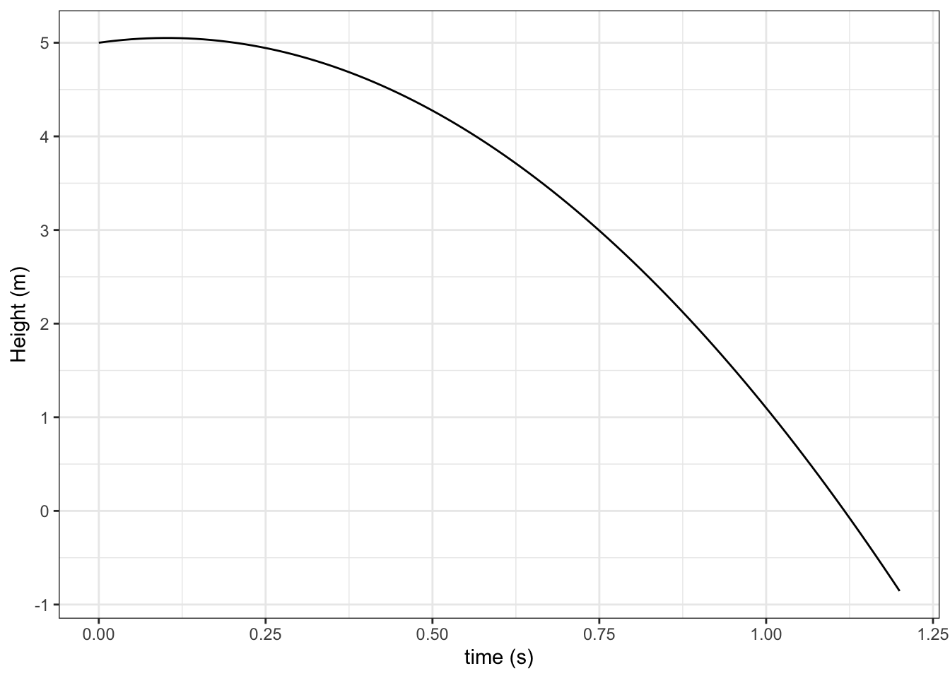
The diver hits the water at about \(t = 1.1\) s. Of course, once in the water, the diver is no longer accelerating downward, so the model isn’t valid for \(x < 0\).
What’s nice about the differential equation format is that it’s easy to add features like the buoyancy of water and drag of the water. We’ll do that here by changing the acceleration (the \(dv\) term) so that when \(x < 0\) the acceleration is slightly positive (buoyant) with a drag term proportional to \(v^2\) in the direction opposed to the motion.
diveFloat <- integrateODE(
        dv ~ ifelse(x <  0, 1 - 2 * sign(v) * v^2, -9.8),
        dx ~ v,
        v = 1, x = 5, tdur = 10)
slice_plot(diveFloat$x(t) ~ t, domain(t = 0:10)) %>%
  gf_labs(ylab="Height (m)", xlab="time (s)")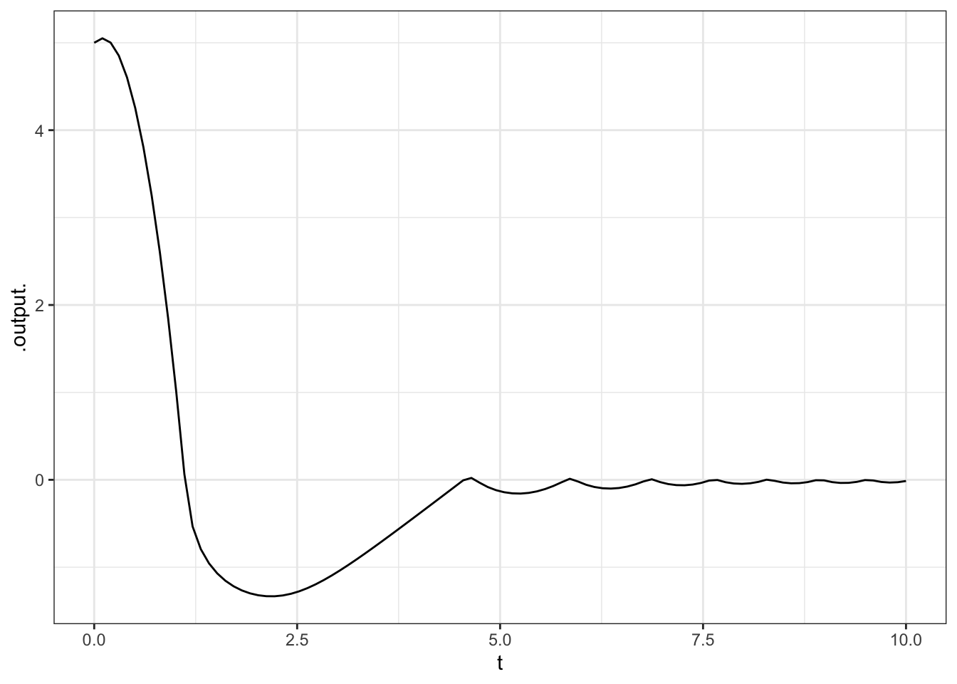
According to the model, the diver resurfaces at about 5 seconds, and then bobs in the water.
9.2.2 Exercises
9.2.2.1 Exercise 1
FIX FIX FIX Get the exercises from the final version of the book FIX FIX FIX An equation for exponential growth. What’s the value at time \(t = 10\)?
9.2.2.2 Exercise 2
An equation for logistic growth. What’s the value at time \(t = 10\)?
9.2.2.3 Exercise 3
A phase plane problem.
9.2.2.4 Exercise 4
Linear phase plane. Ask about different parameters. Is the system stable or unstable; oscillatory or not?
9.2.2.5 Exercise 5
Or maybe move to an activity. The diving model. Vary the parameters until the maximum depth is some specified value.
We need to be more specific about dollars, because there are US dollars, Australian dollars, New Zealand dollars, Fijian dollars, Namimbian dollars and many others.↩︎
Highly experienced R programmers will recognize that this statement is only partially correct. A complete statement involves a computer-language concept called “scoping.” We’ll have another footnote later when we introduce
makeFun(). You experts might want to keep an eye out for it.↩︎Pick up on the footnote for experts in chapter 1, explain how the parameters are carried along with the function and not variables in the global environment. In terms of the computer language, we don’t distinguish between parameters and variables.↩︎
In traditional notation, the formula is prettier: \[x(t) = \frac{K x_0}{x_0 + (K − x_0 e^{−rt})}.\] The parentheses in computer notation attract more than their fair share of visual attention when attached to single-letter variables like \(x\).↩︎