Chapter 1 Representing mathematical functions
As the title suggests, in this book we are going to be using the R computer language to implement the operations of calculus along with related operations such as graphing and solving.
The topic of calculus is fundamentally about mathematical functions and the operations that are performed on them. The concept of “mathematical function” is an idea. If we are going to use a computer language to work with mathematical functions, we will need to translate them into some entity in the computer language. That is, we need a language construct to represent functions and the quantities functions take as input and produce as output.
If you happen to have a background in programming, you may well be thinking that the choice of representation is obvious. For quantities, use numbers. For functions, use R-language functions. That is indeed what we are going to do, but as you’ll see, the situation is just a little more complicated than that. A little, but that little complexity needs to be dealt with from the beginning.
1.1 Numbers, quantities, and names
The complexity mentioned in the previous section stems the uses and real-world situations to which we want to be able to apply the mathematical idea of functions. The inputs taken by functions and the outputs produced by them are not necessarily numbers. Often, they are quantities.
Consider these examples of quantities: money, speed, blood pressure, height, volume. Isn’t each of these quantities a number? Not quite. Consider money. We can count, add, and subtract money – just like we count, add, and subtract with numbers. But money has an additional property: the kind of currency. There are Dollars1, Renminbi, Euros, Rand, Krona and so on. Money as an idea is an abstraction of the kind sometimes called a dimension. Other dimensions are length, time, volume, temperature, area, angle, luminosity, bank interest rate, and so on. When we are dealing with a quantity that has dimension, it’s not enough to give a number to say “how much” of that dimension we have. We need also to give units. Many of these are familiar in everyday life. For instance, the dimension of length is quantified with units of meters, or inches, or miles, or parsecs, and so on. The dimension of money is measured with euros, dollars, renminbi, and so on. Area as a dimension is quantified with square-meters, or square-feet, or hectares, or acres, etc.
Unfortunately, most mathematics texts treat dimension and units by ignoring them. This leads to confusion and error when an attempt is made to apply mathematical ideas to quantities in the real world.
In this book we will be using functions and calculus to work with real-world quantities. We can’t afford to ignore dimension and units. Unfortunately, mainstream computer languages like R and Python and JavaScript do not provide a systematic way to deal with dimension and units automatically. In R, for example, we can easily write
which stores a quantity under the name x. But the language bawks at something like
## Error: <text>:1:9: unexpected symbol
## 1: y <- 12 meters
##             ^
Lacking a proper computer notation for representing dimensioned quantities with their units, we need some other way to keep track of things.
Here is what we will do. When we represent a quantity on the computer, we will use the name of the quantity to remind us what the dimension and units are. Suppose we want, for instance, to represent a family’s yearly income. A sensible choice is to use names like income or income_per_year or family_income. We might even give the units in the name, e.g. family_income_euros_per_year. But usually what we do is to document the units separately for a human reader.
This style of using the name of a quantity as a reminder of the dimension and units of the quantity is outside the tradition of mathematical notation. In high-school math, you encountered \(x\) and \(y\) and \(t\) and \(\theta\). You might even have seen subscripts used to be more specific, for instance \(x_0\). Someone trained in physics will know the traditional and typical uses of letters. \(x\) is likely a position, \(t\) is likely a time, and \(x_0\) is the position at time zero.
In many areas of application, there are many different quantities to be represented. To illustrate, consider a textbook about the turbulent flow of fluids: Turbulent Flows by Stephen B. Pope (ISBN 978-0521598866). In the book’s prefatory matter, there is a 14-page long section entitled “Nomenclature.” Figure 1.1 shows a small part of that section, just the symbols that start with the capital letters R and S.
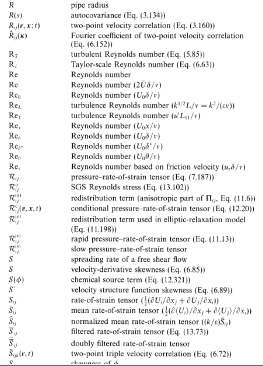
Figure 1.1: Part of one page from the 14-page long nomenclature section of Turbulent Flows by Stephen B. Pope
Each page in the nomenclature section is dense with symbols. The core of most of them is one or two letters, e.g. \(R\) or \(Re\). But there are only so many letters available, even if Greek and other alphabets are brought into things. And so more specificity is added by using subscripts, superscripts, hats (e.g. \(\hat{S}_{ij}\)), bars (e.g. \(\bar{S}_{ij}\)), stars, and so on. My favorite on this page is \(Re_{\delta^\star}\) in which the subscript \(\delta^\star\) itself has a superscript \(^\star\).
For experts working extensively with algebraic manipulations, this elaborate system of nomenclature may be unavoidable and even optimal. But when the experts are implementing their ideas as computer programs, they have to use a much more mundane approach to naming things: character strings like Reynolds.
There can be an advantage to the mundane approach. In this book, we’ll be working with calculus, which is used in a host of fields. We’re going to be drawing examples from many fields. And so we want our quantities to have names that are easy to recognize and remember. Things like income and blood_pressure and farm_area. If we tried to stick to x and y and z, our computer notation would become incomprehensible to the human reader and thus easily subject to error.
1.2 R-language functions
R, like most computer languages, has a programming construct to represent operations that take one or more inputs and produce an output. In R, these are called “functions.” In R, everything you do involves a function, either explicitly or implicitly.
Let’s look at the R version of a mathematical function, exponentiation. The function is named exp and we can look at the programming it contains
## function (x) .Primitive("exp")Not much there, except computer notation. In R, functions can be created with the key word function. For instance, to create a function that translates yearly income to daily income, we could write:
The name selected for the function, as_daily_income, is arbitrary. We could have named the function anything at all. (It’s a good practice to give functions names that are easy to read and write and remind you what they are about.)
After the keyword function, there is a pair of parentheses. Inside the parentheses are the names being given to the inputs to the function. There’s just one input to as_daily_income which we called yearly_income just to help remind us what the function is intended to do. But we could have called the input anything at all.
The part function(yearly_income) specifies that the thing being created will be a function and that we are calling the input yearly_income. After this part comes the body of the function. The body contains R expressions that specify the calculation to be done. In this case, the expression is very simple: divide yearly_income by 365 – the (approximate) number of days in a year.
It’s helpful to distinguish between the value of an input and the role that the input will play in the function. A value of yearly income might be 61362 (in, say, dollars). To speak of the role that the input plays, we use the word argument. For instance, we might say something like, “as_yearly_income is a function that takes one argument.”
Following the keyword function and the parentheses where the arguments are defined comes a pair of curly braces { and } containing some R statements. These statements are the body of the function and contain the instructions for the calculation that will turn the inputs into the output.
Here’s a surprising feature of computer languages like R … The name given to the argument doesn’t matter at all, so long as it is used consistently in the body of the function. So the programmer might have written the R function this way:
or even
All of these different versions of as_daily_income() will do exactly the same thing and be used in exactly the same way, regardless of the name given for the argument.2 Like this:
## [1] 168.1151Often, functions have more than one argument. The names of the arguments are listed between the parentheses following the keyword function, like this:
In such a case, to use the function we have to provide all the arguments. So, with the most recent two-argument definition of as_daily_income(), the following use generates an error message:
## Error in as_daily_income(61362): argument "duration" is missing, with no defaultInstead, specify both arguments:
## [1] 168.1151One more aspect of function arguments in R … Any argument can be given a default value. It’s easy to see how this works with an example:
With the default value for duration the function can be used with either one argument or two:
## [1] 168.1151## [1] 167.6557The second line is the appropriate calculation for a leap year.
To close, let’s return to the exp function, which is built-in to R. The single argument to exp was named x and the body of the function is somewhat cryptic: .Primitive("exp").
It will often be the case that the functions we create will have bodies that don’t involve traditional mathematical expressions like \(x / d\). As you’ll see in later chapters, in the modern world many mathematical functions are too complicated to be represented by algebraic notation.
Don’t be put off by such non-algebra function bodies. Ultimately, what you need to know about a function in order to use it are just three things:
- What are the arguments to the function and what do they stand for.
- What kind of thing is being produced by the function.
- That the function works as advertised, e.g. calculating what we would write algebraically as \(e^x\).
1.3 Literate use of arguments
Recall that the names selected by the programmer of a function are arbitrary. You would use the function in exactly the same way even if the names were different. Similarly, when using the function you can pick yourself what expression will be the value of the argument.
For example, suppose you want to calculate \(100 e^{-2.5}\). Easy:
## [1] 8.2085But it’s likely that the \(-2.5\) is meant to stand for something more general. For instance, perhaps you are calculating how much of a drug is still in the body ten days after a dose of 100 mg was administered. There will be three quantities involved in even a simple calculation of this: the dosage, the amount of time since the dose was taken, and what’s called the “time constant” for elimination of the drug via the liver or other mechanisms. (To follow this example, you don’t have to know what a time constant is. But if you’re interested, here’s an example. Suppose a drug has a time constant of 4 days. This means that a 63% of the drug will be eliminated during a 4-day period.)
In writing the calculation, it’s a good idea to be clear and explicit about the meaning of each quantity used in the calculation. So, instead of 100 * exp(-2.5), you might want to write:
dose <- 100 # mg
duration <- 10 # days
time_constant <- 4 # days
dose * exp(- duration / time_constant)
## [1] 8.2085Even better, you could define a function that does the calculation for you:
drug_remaining <- function(dose, duration, time_constant) {
  dose * exp(- duration / time_constant)
}
Then, doing the calculation for the particular situation described above is a matter of using the function:
## [1] 8.2085By using good, descriptive names and explicitly labelling which argument is which, you produce a clear and literate documentation of what you are intending to do and how someone else, including “future you,” should change things for representing a new situation.
1.4 With respect to …
We’ve been using R functions to represent the calculation of quantities from inputs like the dose and time constant of a drug.
But R functions play a much bigger role than that. Functions are used for just about everything, from reading a file of data to drawing a graph to finding out what kind of computer is being used. Of particular interest to us here is the use of functions to represent and implement the operations of calculus. These operations have names that you might or might not be familiar with yet: differentiation, integration, etc.
When a calculus or similar mathematical operation is being undertaken, you usually have to specify which variable or variables the operation is being done “with respect to.” To illustrate, consider the conceptually simple operation of drawing a graph of a function. More specifically, let’s draw a graph of how much drug remains in the body as a function of time since the dose was given. The basic pharmacokinetics of the process is encapsulated in the drug_remaining() function. So what we want to do is draw a graph of drug_remaining().
Recall that drug_remaining() has three arguments: dose, duration, and time_constant. The particular graph we are going to draw shows the drug remaining as a function of duration. That is, the operation of graphing will be with respect to duration. We’ll consider, say, a dose of 100 mg of a drug with a time constant of 4 days, looking perhaps at the duration interval from 0 days to 20 days.
In this book, we’ll be using operations provided by the mosaic and mosaicCalc packages for R. The operations from these packages have a very specific notation to express with respect to. That notation uses the tilde character, ~. Here’s how to draw the graph we want, using the package’s slice_plot() operation:
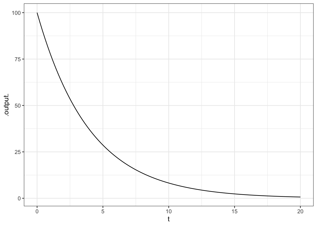
A proper graph would be properly labelled, for instance the horizontal axis with “Time (days)” and the vertical axis with “Remaining drug (mg)”. You’ll see how to do that in the next chapter, which explores the function-graphing operation in more detail.