Chapter 3 Parameters and functions
3.1 Parameters versus variables
Why there’s not really a difference.
Newton’s distinction between a, b, c, and x, y, z.
3.2 Parameters of modeling functions
Give the parameterizations of exponentials, sines, power laws …
The idea is to make the arguments to the mathematical functions dimensionless.
Parameters and logarithms – You can take the log of anything you like. The units show up as a constant
3.3 Polynomials and parameters
Each parameter has its own dimension
3.4 Parameters and makeFun()
Describe how makeFun() works here.1
3.5 Functions without parameters: splines and smoothers
EXPLAIN hyper-parameter. It’s a number that governs the shape of the function, but it can be set arbitrarily and still match the data. Hyper-parameters are not set directly by the data.
Mathematical models attempt to capture patterns in the real world. This is useful because the models can be more easily studied and manipulated than the world itself. One of the most important uses of functions is to reproduce or capture or model the patterns that appear in data.
Sometimes, the choice of a particular form of function — exponential or power-law, say — is motivated by an understanding of the processes involved in the pattern that the function is being used to model. But other times, all that’s called for is a function that follows the data and that has other desirable properties, for example is smooth or increases steadily.
“Smoothers” and “splines” are two kinds of general-purpose functions that can capture patterns in data, but for which there is no simple algebraic form. Creating such functions is remarkably easy, so long as you can free yourself from the idea that functions must always have formulas.
Smoothers and splines are defined not by algebraic forms and parameters, but by data and algorithms. To illustrate, consider some simple data. The data set Loblolly contains 84 measurements of the age and height of loblolly pines.
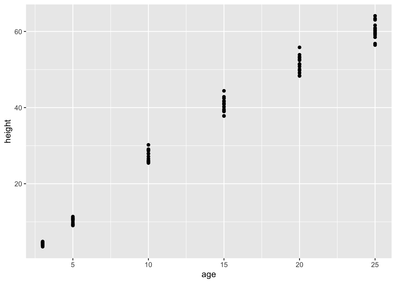
Several three-year old pines of very similar height were measured and tracked over time: age five, age ten, and so on. The trees differ from one another, but they are all pretty similar and show a simple pattern: linear growth at first which seems to low down over time.
It might be interesting to speculate about what sort of algebraic function the loblolly pines growth follows, but any such function is just a model. For many purposes, measuring how the growth rate changes as the trees age, all that’s needed is a smooth function that looks like the data. Let’s consider two:
- A “cubic spline”, which follows the groups of data points and curves smoothly and gracefully.
- A “linear interpolant”, which connects the groups of data points with straight lines.
The definitions of these functions may seem strange at first — they are entirely defined by the data: no parameters! Nonetheless, they are genuine functions and can be worked with like other functions. For example, you can put in an input and get an output:
## [1] 20.68193## [1] 20.54729You can graph them:
gf_point(height ~ age, data = datasets::Loblolly) %>%
  slice_plot(f1(age) ~ age) %>%
slice_plot(f2(age) ~ age, color="red", ) 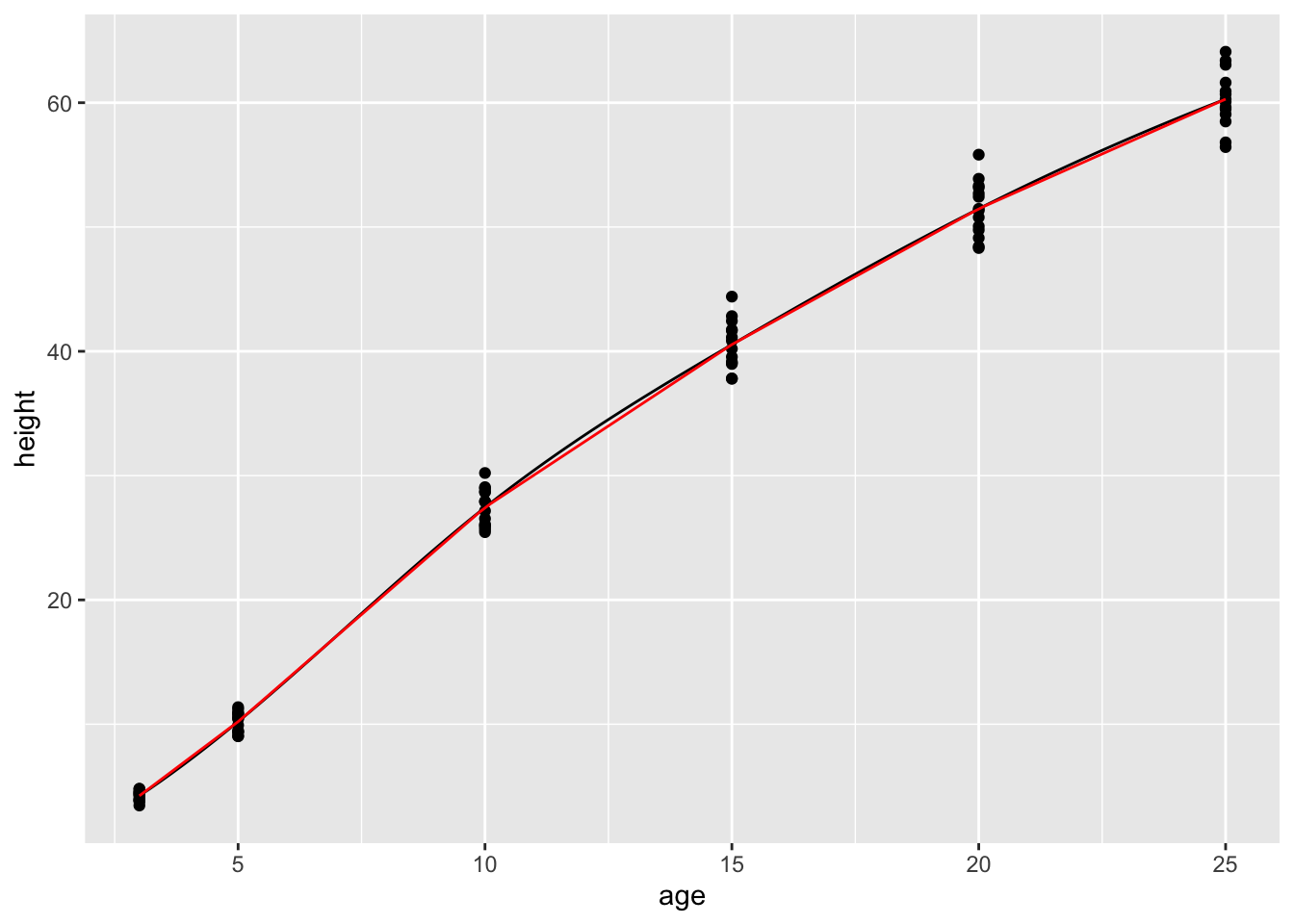
You can even “solve” them, for instance finding the age at which the height will be 35 feet:
##       age
## 1 12.6905## age
## 1 12.9In all respects, these are perfectly ordinary functions. All respects but one: there is no simple formula for them. You’ll notice this if you ever try to look at the computer-language definition of the functions:
## function (age)
## {
##     x <- get(fnames[2])
##     if (connect)
##         SF(x)
##     else SF(x, deriv = deriv)
## }
## <environment: 0x7ff1bf85ec18>
There’s almost nothing here to tell the reader what the body of the function is doing. The definition refers to the data itself which has been stored in an “environment.” These are computer-age functions, not functions from the age of algebra.
As you can see, the spline and linear connector functions are quite similar, except for the range of inputs outside of the range of the data. Within the range of the data, however, both types of functions go exactly through the center of each age-group.
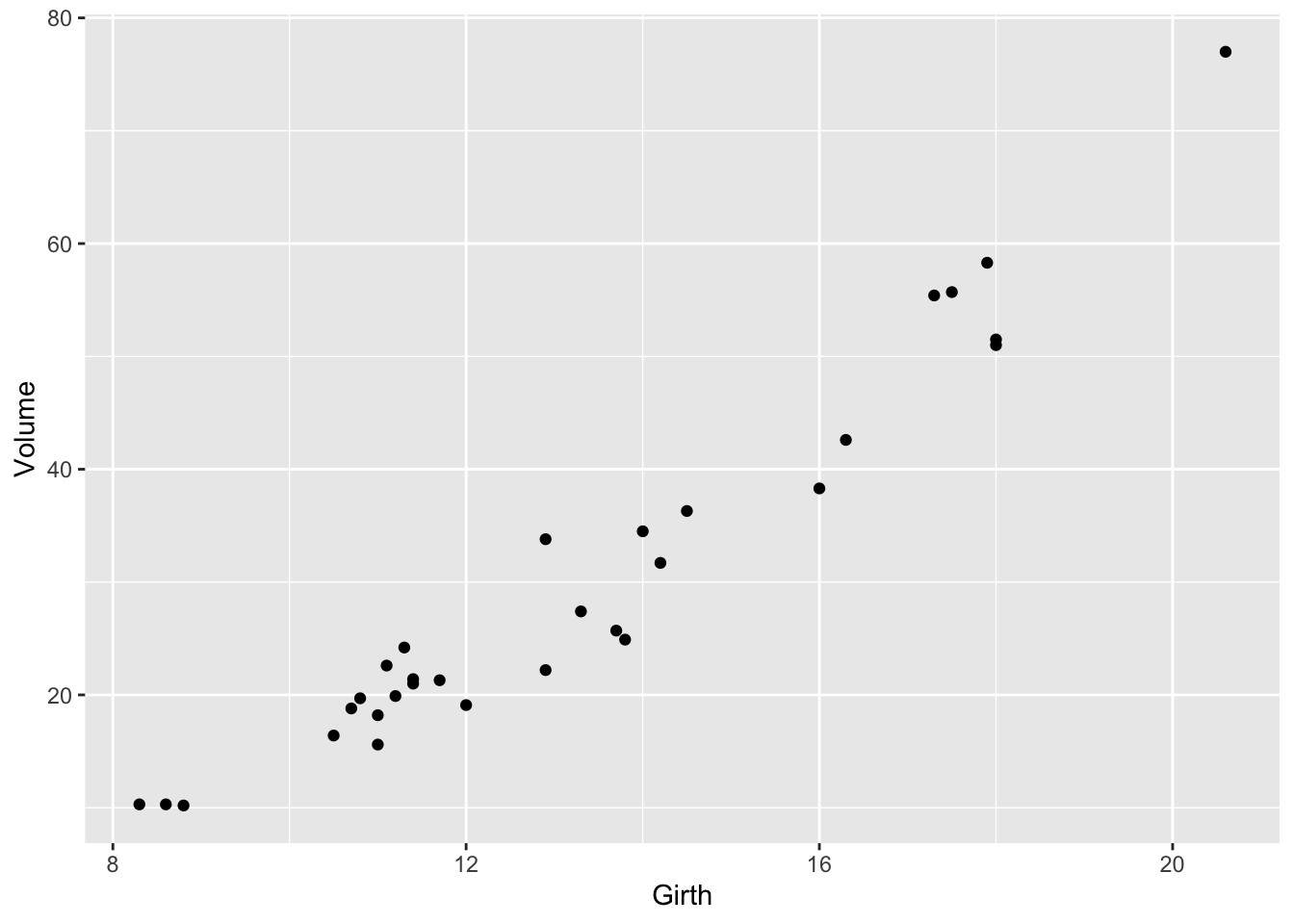
Splines and connectors are not always what you will want, especially when the data are not divided into discrete groups, as with the loblolly pine data. For instance, the trees.csv data set is measurements of the volume, girth, and height of black cherry trees. The trees were felled for their wood, and the interest in making the measurements was to help estimate how much usable volume of wood can be gotten from a tree, based on the girth (that is, circumference) and height. This would be useful, for instance, in estimating how much money a tree is worth. However, unlike the loblolly pine data, the black cherry data does not involve trees falling nicely into defined groups.
It’s easy enough to make a spline or a linear connector:
g1 = spliner(Volume ~ Girth, data = Cherry)
g2 = connector(Volume ~ Girth, data = Cherry)
slice_plot(g1(x) ~ x, domain(x = 8:18)) %>%
  slice_plot(g2(x) ~ x, color ="red") %>%
  gf_point(Volume ~ Girth, data = Cherry) %>%
  gf_labs(x = "Girth (inches)")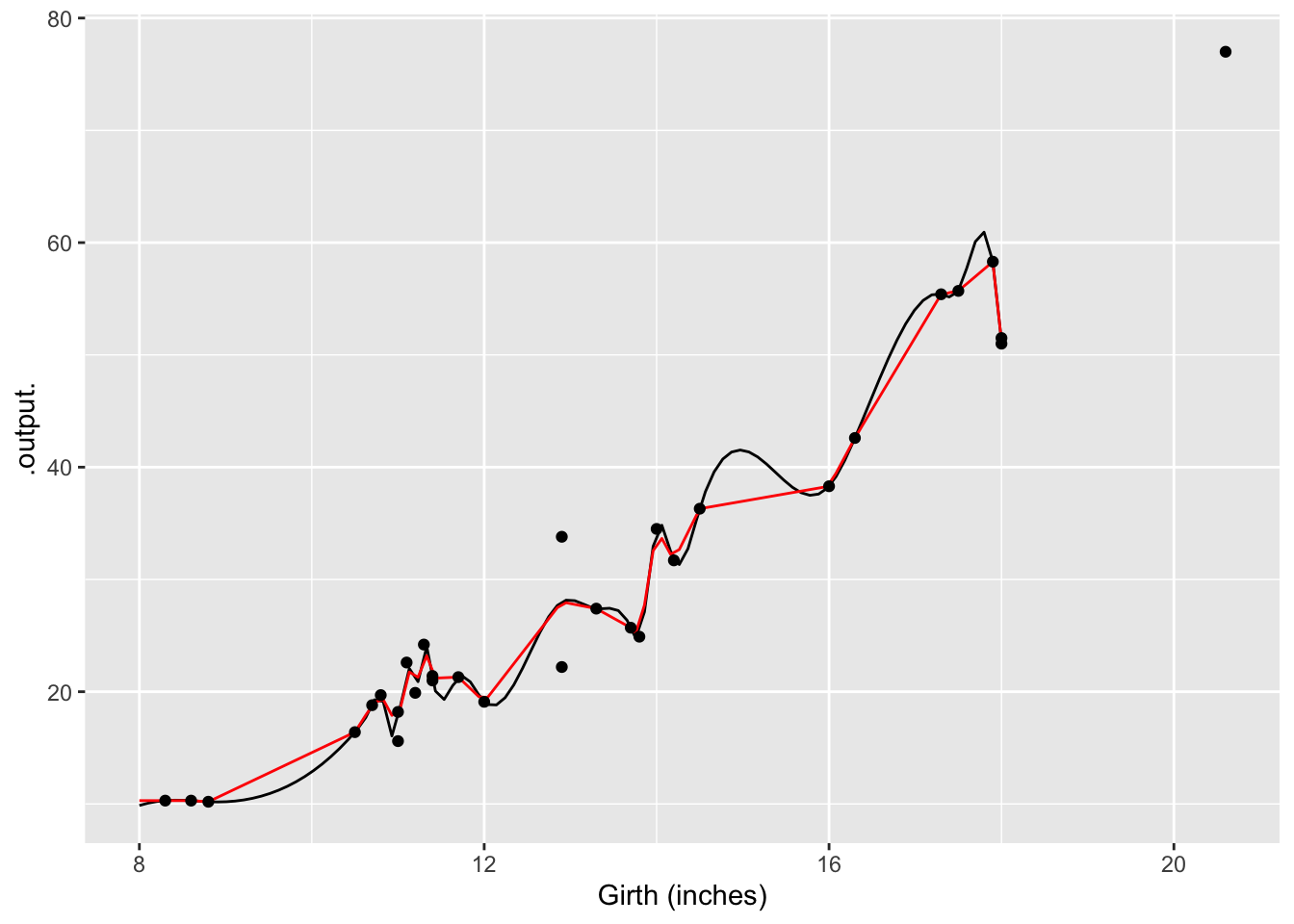
The two functions both follow the data … but a bit too faithfully! Each of the functions insists on going through every data point. (The one exception is the two points with girth of 13 inches. There’s no function that can go through both of the points with girth 13, so the functions split the difference and go through the average of the two points.)
The up-and-down wiggling is of the functions is hard to believe. For such situations, where you have reason to believe that a smooth function is more appropriate than one with lots of ups-and-downs, a different type of function is appropriate: a smoother.
g3 <- smoother(Volume ~ Girth, data = Cherry, span=1.5)
gf_point(Volume~Girth, data=Cherry) %>%
  slice_plot(g3(Girth) ~ Girth) %>%
  gf_labs(x = "Girth (inches)")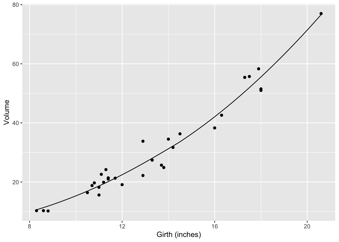
Smoothers are well named: they construct a smooth function that goes close to the data. You have some control over how smooth the function should be. The hyper-parameter span governs this:
g4 <- smoother(Volume ~ Girth, data=Cherry, span=1.0)
gf_point(Volume~Girth, data = Cherry) %>%
  slice_plot(g4(Girth) ~ Girth) %>%
  gf_labs(x = "Girth (inches)", y = "Wood volume")
Of course, often you will want to capture relationships where there is more than one variable as the input. Smoothers do this very nicely; just specify which variables are to be the inputs.
g5 <- smoother(Volume ~ Girth+Height,
               data = Cherry, span = 1.0)
gf_point(Height ~ Girth, data = Cherry) %>%
  contour_plot(g5(Girth, Height) ~ Girth + Height) %>%
  gf_labs(x = "Girth (inches)",
          y = "Height (ft)",
          title = "Volume (ft^3)")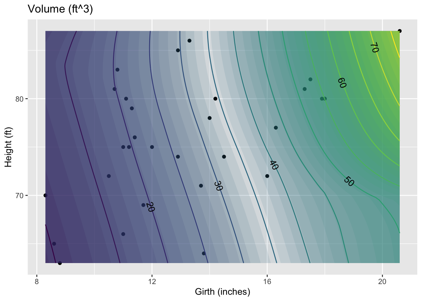
When you make a smoother or a spline or a linear connector, remember these rules:
- You need a data frame that contains the data.
- You use the formula with the variable you want as the output of the function on the left side of the tilde, and the input variables on the right side.
- The function that is created will have input names that match the variables you specified as inputs. (For the present, only
smootherwill accept more than one input variable.) - The smoothness of a
smootherfunction can be set by thespanargument. A span of 1.0 is typically pretty smooth.The de fault is 0.5. - When creating a spline, you have the option of declaring
monotonic=TRUE. This will arrange things to avoid extraneous bumps in data that shows a steady upward pattern or a steady downward pattern.
When you want to plot out a function, you need of course to choose a range for the input values. It’s often sensible to select a range that corresponds to the data on which the function is based. You can find this with the range() command, e.g.
## [1] 63 87