Chapter 8 Integrals and integration

You’ve already seen a fundamental calculus operator, differentiation, which is implement by the R/mosaicCalc function D(). The diffentiation operator takes as input a function and a “with respect to” variable. The output is another function which has the “with respect to” variable as an argument, and potentially other arguments as well.

f <- makeFun( A * x ^  2 ~ x, A = 0.5)
f(1)

## [1] 0.5

f(2)

## [1] 2

f(3)

## [1] 4.5

df <- D(f(x) ~ x)
df(1)

## [1] 1

df(2)

## [1] 2

df(3)

## [1] 3

slice_plot(f(x) ~ x, domain(x = -1:1)) %>%
  gf_labs(title = "Original function f(x)")
slice_plot(df(x) ~ x, domain(x =-1:1), color = "red") %>%
  gf_labs(title = "New function df(x), the derivative of f(x)")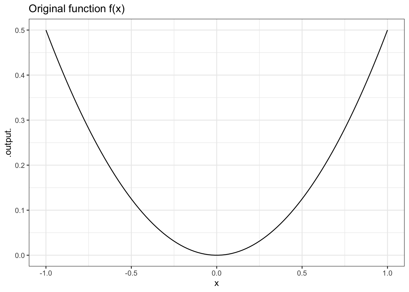

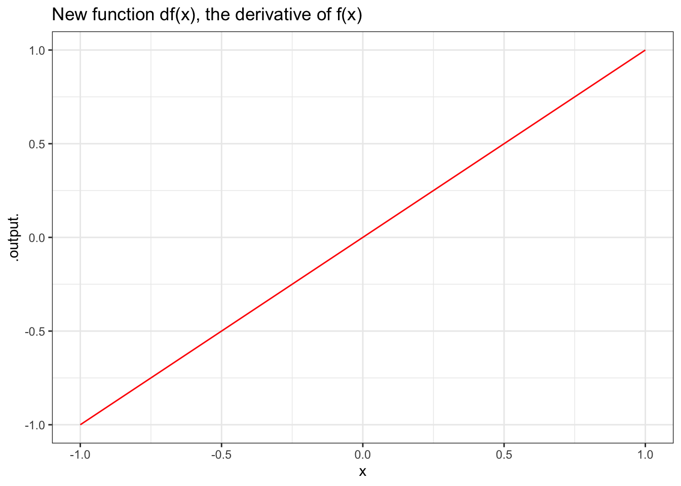
Figure 8.1: A function and its derivative.

Figure 8.1 shows a graph of \(f(x)\) – a smiley curve – and its derivative \(df(x)\).

8.1 The anti-derivative

Now, imagine that we start with \(df(x)\) and we want to find a function \(DF(x)\) where the derivative of \(DF(x)\) is \(f(x)\). In other words, imagine applying the inverse of the \(D()\) operator to the function \(df(x)\) produces \(f()\) (or something much like it).

This inverse operator is implemented in R/mosaicCalc as the antiD() function. As the suffix anti suggests, antiD() “undoes” the what \(D()\) does. Like this:

DF <- antiD(df(x) ~ x)
DF(1)

## [1] 0.5

DF(2)

## [1] 2

DF(3)

## [1] 4.5

slice_plot(df(x) ~ x, domain(x=-1:1), color = "red") %>%
  gf_labs(title = "Original function df(x)")
slice_plot(DF(x) ~ x, domain(x=-1:1)) %>%
  gf_labs(title = "New function DF(x), the anti-derivative of df(x)")

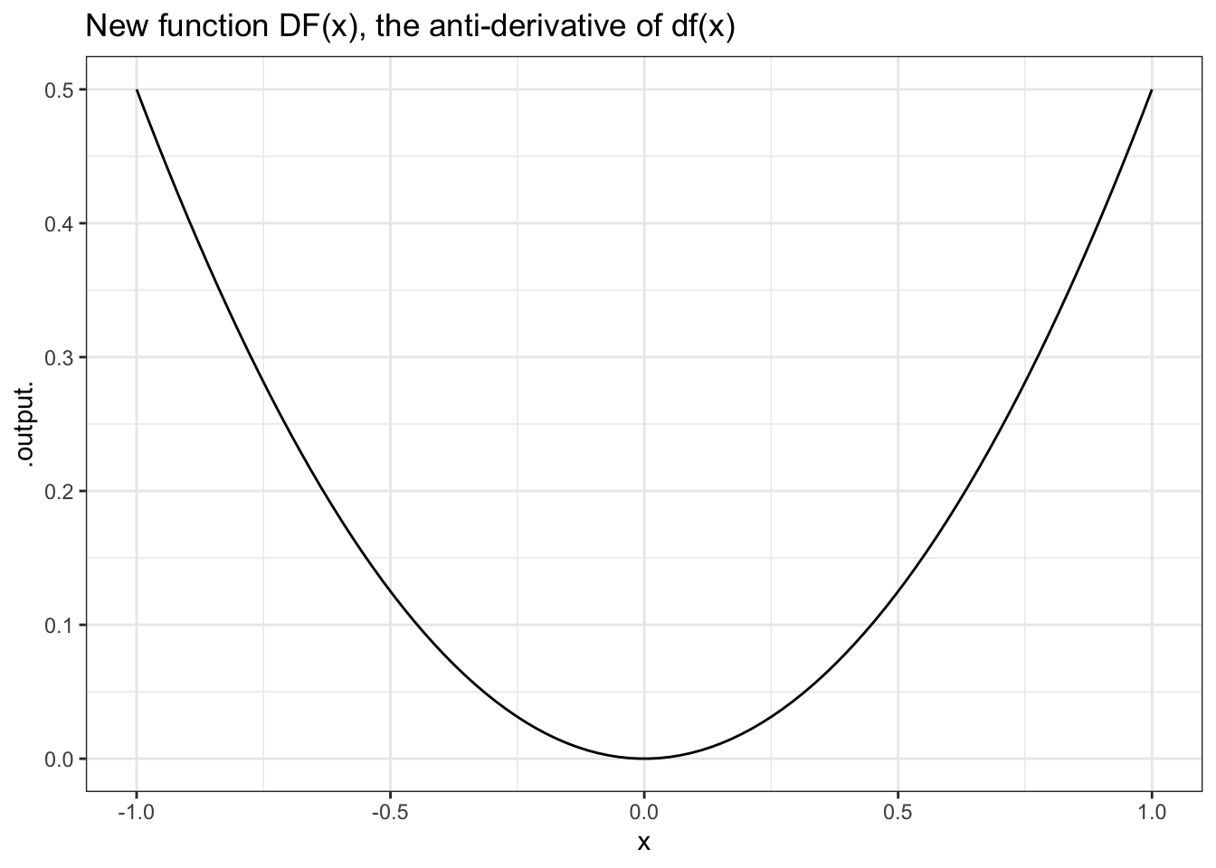
Figure 8.2: A function and its anti-derivative.

Notice that the function \(DF\) was created by anti-differentiating not \(f\) but \(df\) with respect to \(x\). The result is a function that’s “just like” \(f\). (Why the quotes on “just like”? You’ll see.) You can see that the values of \(DF\) are the same as the values of the original \(f\).

You can also go the other way: anti-differentiating a function and then taking the derivative to get back to the original function.

h <- antiD( f(x) ~ x )
dh <- D(h(x) ~ x )
dh(1)

## [1] 0.5

dh(2)

## [1] 2

dh(3)

## [1] 4.5

As you can see, antiD( ) undoes D( ), and D( ) undoes antiD( ). It’s that easy. But there is one catch: for any function \(f(x)\) there are many anti-derivatives of \(f(x)\).

8.2 One variable becomes two arguments

It’s rarely the case that you will want to anti-differentiate a function that you have just differentiated. One undoes the other, so there is little point except to illustrate in a textbook how differentiation and anti-differentiation are related to one another. But it often happens that you are working with a function that describes the derivative of some unknown function, and you wish to find the unknown function.

This is often called “integrating” a function. “Integration” is a shorter and nicer term than “anti-differentiation,” and is the more commonly used term. The function that’s produced by the process is generally called an “integral.” The terms “indefinite integral” and “definite integral” are often used to distinguish between the function produced by anti-differentiation and the value of that function when evaluated at specific inputs. This will be confusing at first, but you’ll soon get a feeling for what’s going on.

As you know, a derivative tells you a local property of a function: how the function changes when one of the inputs is changed by a small amount. The derivative is a sort of slope. If you’ve ever stood on a hill, you know that you can tell the local slope without being able to see the whole hill; just feel what’s under your feet.

An anti-derivative undoes a derivative, but what does it mean to “undo” a local property? The answer is that an anti-derivative (or, in other words, an integral) tells you about some global or distributed properties of a function: not just the value at a point, but the value accumulated over a whole range of points. This global or distributed property of the anti-derivative is what makes anti-derivatives a bit more complicated than derivatives, but not much more so.

At the core of the problem is that there is more than one way to “undo” a derivative. Consider the following functions, each of which is different:

f1 <- makeFun(sin(x ^ 2) ~ x)
f2 <- makeFun(sin(x ^ 2)  +  3 ~ x)
f3 <- makeFun(sin(x ^ 2)  -  100 ~ x)
f1(1)

## [1] 0.841471

f2(1)

## [1] 3.841471

f3(1)

## [1] -99.15853

Despite the fact that the functions \(f_1(x)\), \(f_2(x)\), and \(f_3(x)\), are different, they all have the same derivative.

df1 = D(f1(x) ~ x)
df2 = D(f2(x) ~ x)
df3 = D(f3(x) ~ x)
df1(1)

## [1] 1.080605

df2(1)

## [1] 1.080605

df3(1)

## [1] 1.080605

This raises a problem. When you “undo” the derivative of any of df1, df2, or df3, what should the answer be? Should you get \(f_1\) or \(f_2\) or \(f_3\) or some other function? It appears that the antiderivative is, to some extent, indefinite.

The answer to this question is by no means a philosophical mystery. There’s a very definite answer. Or, rather, there are two answers that work out to be different faces of the same thing.

To start, it helps to review the traditional mathematical notation, so that it can be compared side-by-side with the computer notation. Given a function \(f(x)\), the derivative with respect to \(x\) is written \(df/dx\) and the anti-derivative is written \(\int f(x) dx\).

All of the functions that have the same derivative are similar. In fact, they are identical except for an additive constant. So the problem of indefiniteness of the antiderivative amounts just to an additive constant — the anti-derivative of the derivative of a function will be the function give or take an additive constant: \[ \int \frac{df}{dx} dx = f(x) + C .\] So, as long as you are not concerned about additive constants, the anti-derivative of the derivative of a function gives you back the original function.

8.3 The integral

The derivative tells you how a function changes locally. The anti-derivative accumulates those local values to give you a global value; it considers not just the local properties of the function at a single particular input value but the values over a range of inputs.

Remember that the derivative of \(f\) is itself a function, and that function has the same arguments as \(f\). So, since f(x) was defined to have an argument named x, the function created by D(f(x) ~ x) also has an argument named x (and whatever other parameters are involved):

f

## function (x, A = 0.5) 
## A * x^2
## <bytecode: 0x7fe6038205e0>

df

## function (x, A = 0.5) 
## A * (2 * (x))
## <bytecode: 0x7fe603934720>

The anti-derivative operation is a little bit different in this respect. When you use antiD(), the name of the function’s variable is replaced by two arguments: the actual name (in this example, \(x\)) and the constant \(C\):

antiD(f(x) ~ x)
antiD(df(x) ~ x)

The value of C sets, implicitly, the lower end of the range over which the accumulation is going to occur.

This is a point that is somewhat obscured by traditional mathematical notation, which allows you to write down statements that are not completely explicit. For example, in traditional notation, it’s quite accepted to write an integration statement like this: \[ \int x^2 dx = \frac{1}{3} x^3 . \] This looks like a function of \(x\). But that’s not the whole truth. In fact, the complete statement of the integral involve another argument: C: \[\int x^2 dx = \frac{1}{3} x^3 + C, \] So, really, the value of \(\int x^2 dx\) is a function both of \(x\) and \(C\). In traditional notation, the \(C\) argument is often left out and the reader is expected to remember that \(\int x^2 dx\) is an “indefinite integral.”

Another traditional style for writing an integral is \[ \int ^{\mbox{to}}_{\mbox{from}} x^2 dx = \left. \frac{1}{3} x^3 \right|^{to}_{from} ,\] where the $. |^{to}_{from} $ means that you are to substitute the values of from and to in for \(x\). For instance: \[ \int ^{2}_{-1} x^2 dx = \left. \frac{1}{3} x^3 \right|^{2}_{-1} = \frac{1}{3} 2^3 - \frac{1}{3} (-1)^3 = \frac{9}{3} = 3\] Notice that it doesn’t matter whether the function had been defined in terms of \(x\) or \(y\) or anything else. In the end, the indefinite integral is a function of from and to.

Notice how the calculation of the definite integral involves two applications of the anti-derivative. The definite interval is the difference between the anti-derivative evaluated at to and the anti-derivate evaluated at from. But how do we know what value of \(C\) to provide when calculating a definite integral. The answer is simple: it doesn’t matter what \(C\) is so long as it is the same in both the to and from evaluations of the anti-derivative. The \(C\) in the from calculation cancels out the \(C\) in the to calculation. Since the \(C\)’s cancel out, any value of \(C\) will do. In the software, we choose to use a default value of \(C = 0\)

fun = antiD( x^2 ~ x )
fun

## function (x, C = 0) 
## 1/3 * x^3 + C

When you evaluate the function at specific numerical values for those arguments, you end up with the “definite integral,” a number:

# This doesn't exist yet. FIX FIX FIX
fun(x = 2) - fun(x = -1)

For now, these are the essential things to remember:

1. The antiD( ) function will compute an anti-derivative.
2. Like the derivative, the anti-derivative is always taken with respect to a variable, for instance antiD( x^2 ~ x ). That variable, here x, is called (sensibly enough) the “variable of integration.” You can also say, “the integral with respect to \(x\).”
3. The definite integral is a function of the variable of integration … sort of. To be more precise, the variable of integration appears as an argument in two guises since the definite integral involves two evaluations: one at \(x =\) to and one at \(x =\) from. The bounds defined by from and to are often called the “region of integration.”

The many vocabulary terms used reflect the different ways you might specify or not specify particular numerical values for from and to: “integral,” “anti-derivative,” “indefinite integral,” and “definite integral.” Admittedly, this can be confusing, but that’s a consequence of something important: the integral is about the “global” or “distributed” properties of a function, the “whole.” In contrast, derivatives are about the “local” properties: the "part. The whole is generally more complicated than the part.

You’ll do well if you can remember this one fact about integrals: there are always two arguments that reflect the region of integration: from and to.

8.3.1 Exercises

8.3.1.1 Exercise 1

Find the numerical value of each of the following definite integrals.

1. \(\int^{5}_{2} x^{1.5} dx\)

ANSWER: <<>>= f = antiD( x^1.5 ~ x ) f(from=2,to=5) @

1. \(\int^{10}_{0} sin( x^2 ) dx\)

ANSWER: <<>>= f = antiD(sin(x^2) ~ x) f(from=0,to=10) @

1. \(\int^{4}_{1} e^{2x} dx\)

{0.58,6.32,20.10,27.29,53.60,107.9,1486.8}

ANSWER:

f = integral(exp(2*x) ~ x)
f(from=1,to=4)

1. \(\int^{2}_{-2} e^{2x} dx\)

{0.58,6.32,20.10,27.29,53.60,107.9,1486.8}

ANSWER:

f = integral(exp(2*x) ~ x)
f(from=-2,to=2)

1. \(\int^{2}_{-2} e^{2 | x |} dx\)

{0.58,6.32,20.10,27.29,53.60,107.9,1486.8}

ANSWER:

f = integral(exp(abs(2*x)) ~ x)
f(from=-2,to=2)

8.3.1.2 Exercise 2

There’s a very simple relationship between \(\int^b_a f(x) dx\) and \(\int^a_b f(x) dx\) — integrating the same function \(f\), but reversing the values of from and to.
Create some functions, integrate them, and experiment with them to find the relationship.

1. They are the same value.
2. One is twice the value of the other.
3. One is negative the other.
4. One is the square of the other.

8.3.1.3 Exercise 3

The function being integrated can have additional variables or parameters beyond the variable of integration. To evaluate the definite integral, you need to specify values for those additional variables.

For example, a very important function in statistics and physics is the Gaussian, which has a bell-shaped graph:

gaussian <- 
  makeFun((1/sqrt(2*pi*sigma^2)) * 
            exp( -(x-mean)^2/(2*sigma^2)) ~ x,
          mean=2, sigma=2.5)
slice_plot(gaussian(x) ~ x, domain(x = -5:10)) %>%
  slice_plot(gaussian(x, mean=0, sigma=1) ~ x, color="red")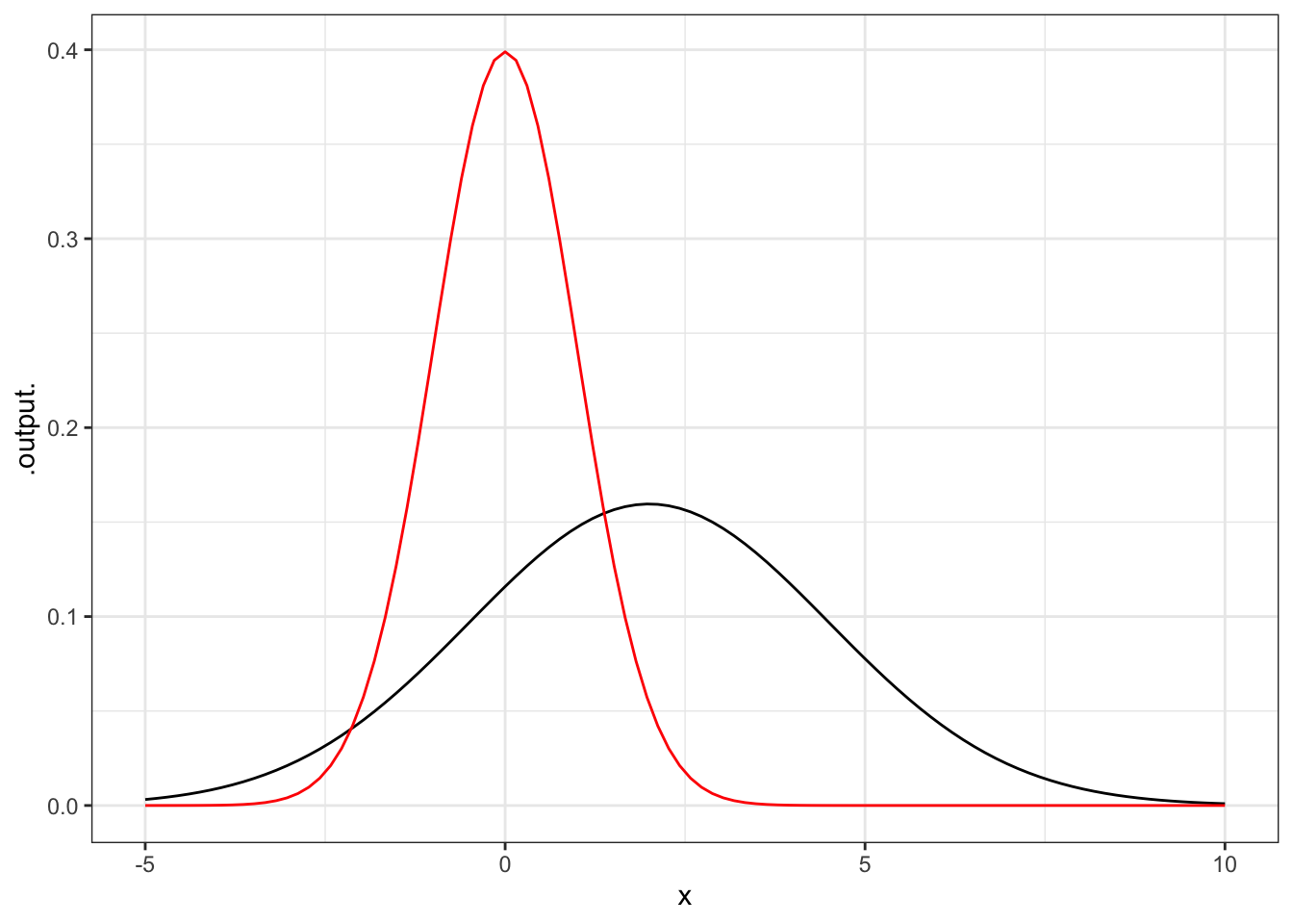

As you can see, it’s a function of \(x\), but also of the parameters mean and sigma.

When you integrate this, you need to tell antiD() or integral() what the parameters are going to be called:

erf <- antiD(gaussian(x, mean=m, sigma=s) ~ x)
erf

Evaluate each of the following definite integrals:

1. \(\int^1_0 \mbox{erf}(x,m=0,s=1) dx\)

{0.13,0.34,0.48,0.50,0.75,1.00}

ANSWER:

erf(x = 1, m=0, s=1) - erf(x = 0, m=0, s=1)

The name erf is arbitrary. In mathematics, erf is the name of something called the ERror Function, just as sin is the name of the sine function. The formal definition of erf is a bit different than the erf presented here, but the name erf is so much fun that I wanted to include it in the book. The real erf is \[ \mbox{erf}_{formal}(x) = 2\ \mbox{erf}_{here}(x) - 1.\]

1. \(\int^2_0 f(x,m=0,s=1) dx\)

{0.13,0.34,0.48,0.50,0.75,1.00}

ANSWER:

erf(x = 2, m=0, s=1) - erf(x = 0, m=0, s=1)

1. \(\int^2_0 f(x,m=0,s=2) dx\)

{-0.48,-0.34,-0.13, 0.13, 0.34, 0.48}

ANSWER:

erf(x = 0, m=0, s=2) - erf(x = 2, m=0, s=2)

1. \(\int^3_{-\infty} f(x,m=3,s=10) dx\). (Hint: The mathematical \(-\infty\) is represented as on the computer.)

{0.13,0.34,0.48,0.50,0.75,1.00}

ANSWER:

erf(x = -Inf, m=3, s=10) - erf(x = 3, m=3, s=10)

1. \(\int^{-\infty}_{\infty} f(x,m=3,s=10) dx\)

{0.13,0.34,0.48,0.50,0.75,1.00}

ANSWER:

erf(x = Inf, m=3, s=10) - erf(x = -Inf, m=3, s=10)