Chapter 5 Fitting nonlinear functions to data

The techniques of linear algebra can be used to find the best linear combination of a set of functions. But, often, there are parameters in functions that appear in a nonlinear way. Examples include $k$ in $f(t) = A \exp( k t ) + C$ and $P$ in $A \sin(\frac{2\pi}{P} t) + C$. Finding these nonlinear parameters cannot be done directly using linear algebra, although the methods of linear algebra do help in simplifying the situation.

Fortunately, the idea that the distance between functions can be measured works perfectly well when there are nonlinear parameters involved. So we’ll continue to use the “sum of square residuals” when evaluating how close an function approximation is to a set of data.

5.1 Exponential functions

To illustrate, consider the data which shows an exponential relationship between the fraction of families with two cars and income:

Families <- read.csv("http://www.mosaic-web.org/go/datasets/Income-Housing.csv")
gf_point(TwoVehicles ~ Income, data = Families)

The pattern of the data suggests exponential “decay” towards close to 100% of the families having two vehicles. The mathematical form of this exponential function is $A exp(k Y) + C$. A and C are unknown linear parameters. $k$ is an unknown nonlinear parameter – it will be negative for exponential decay. Linear algebra allows us to find the best linear parameters $A$ and $C$ in order to match the data. But how to find $k$?

Suppose you make a guess at $k$. The guess doesn’t need to be completely random; you can see from the data themselves that the “half-life” is something like $25,000. The parameter $k$ is corresponds to the half life, it’s $\ln(0.5)/\mbox{half-life}$, so here a good guess for $k$ is $\ln(0.5)/25000$, that is

kguess <- log(0.5) / 25000
kguess

## [1] -2.772589e-05

Starting with that guess, you can find the best values of the linear parameters $A$ and $C$ through linear algebra techniques:

project( TwoVehicles ~ 1 + exp(Income*kguess), data = Families)

##          (Intercept) exp(Income * kguess) 
##             110.4263            -101.5666

Make sure that you understand completely the meaning of the above statement. It does NOT mean that TwoVehicles is the sum $1 + \exp{-\mbox{Income} \times \mbox{kguess}}$. Rather, it means that you are searching for the linear combination of the two functions $1$ and $\exp{-\mbox{Income} \times\mbox{kguess}}$ that matches TwoVehicles as closely as possible. The values returned by tell you what this combination will be: how much of $1$ and how much of $\exp{-\mbox{Income}\times\mbox{kguess}}$ to add together to approximate TwoVehicles.

You can construct the function that is the best linear combination by explicitly adding together the two functions:

f <- makeFun( 110.43 - 101.57*exp(Income * k) ~ Income, k = kguess)
graphFun(f(Income) ~ Income, Incomelim = range(0,100000)) %>%
  gf_point(TwoVehicles ~ Income, data = Families)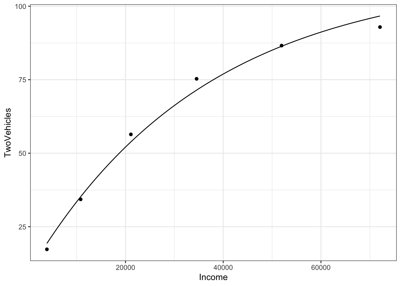

The graph goes satisfyingly close to the data points. But you can also look at the numerical values of the function for any income: <<>>= f(Income=10000) f(Income=50000) @

It’s particularly informative to look at the values of the function for the specific Income levels in the data used for fitting, that is, the data frame Families:

Results <- Families %>% 
  dplyr::select(Income, TwoVehicles) %>%
  mutate(model_val = f(Income = Income),
         resids = TwoVehicles - model_val)
Results

##   Income TwoVehicles model_val     resids
## 1   3914        17.3  19.30528 -2.0052822
## 2  10817        34.3  35.17839 -0.8783904
## 3  21097        56.4  53.84097  2.5590313
## 4  34548        75.3  71.45680  3.8432013
## 5  51941        86.6  86.36790  0.2320981
## 6  72079        92.9  96.66273 -3.7627306

The residuals are the difference between these model values and the actual values of TwoVehicles in the data set.

The resids column gives the residual for each row. But you can also think of the resids column as a vector. Recall that the square-length of a vector is the sum of squared residuals

sum(Results$resids^2)

## [1] 40.32358

This square length of the resids vector is an important way to quantify how well the model fits the data.

5.2 Optimizing the guesses

Keep in mind that the sum of square residuals is a function of $k$. The above value is just for our particular guess $k = $kguess. Rather than using just one guess for $k$, you can look at many different possibilities. To see them all at the same time, let’s plot out the sum of squared residuals as a function of $k$. We’ll do this by building a function that calculates the sum of square residuals for any given value of $k$.

sum_square_resids <- Vectorize(function(k) {
  sum((Families$TwoVehicles - f(Income=Families$Income, k)) ^ 2)
})
graphFun(
   sum_square_resids(k) ~ k, 
   klim = range(log(0.5)/40000,log(0.5)/20000))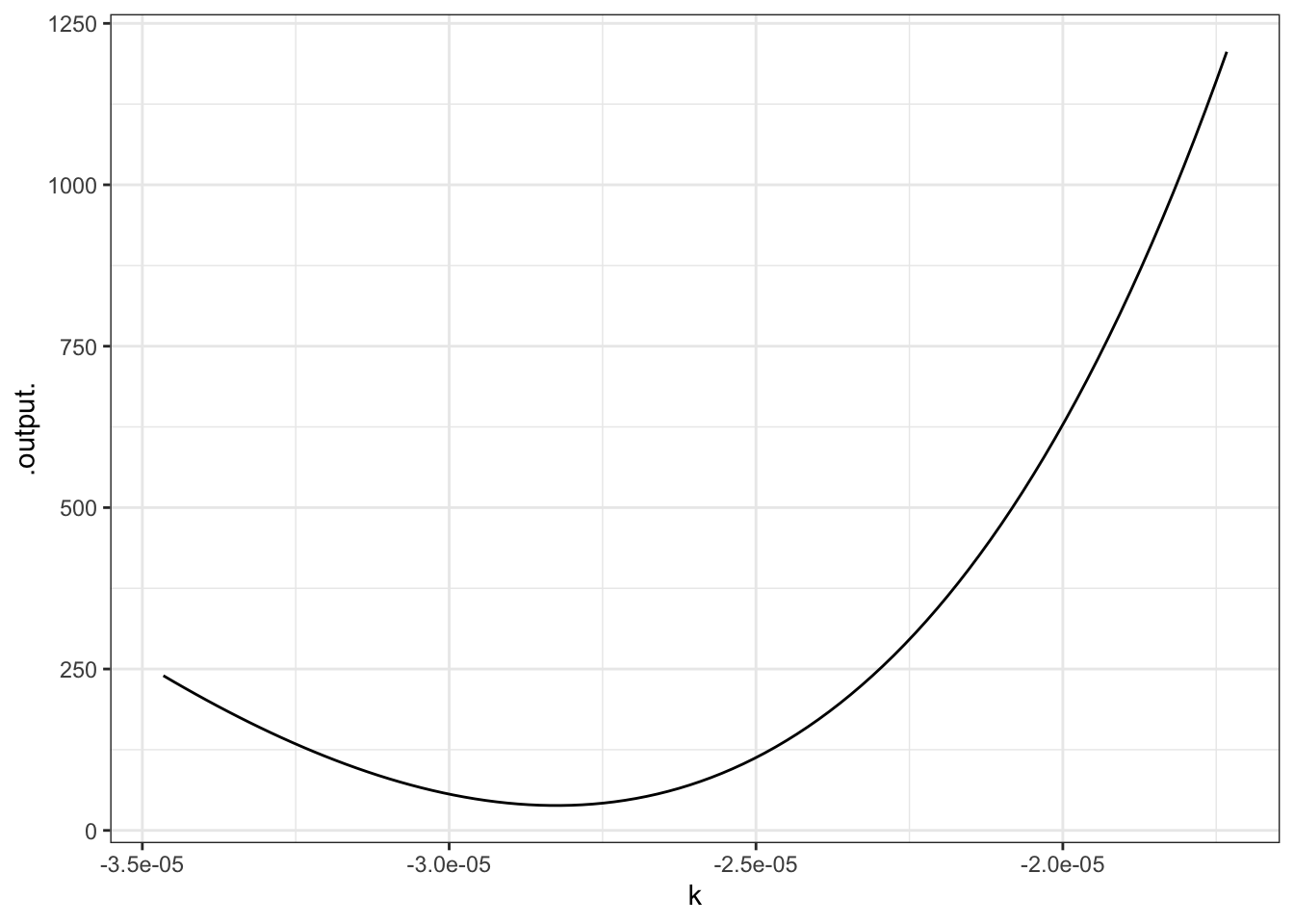

This is a rather complicated computer command, but the graph is straightforward. You can see that the “best” value of $k$, that is, the value of $k$ that makes the sum of square residuals as small as possible, is near $k=-2.8\times10^{-5}$ — not very far from the original guess, as it happens. (That’s because the half-life is very easy to estimate.)

To continue your explorations in nonlinear curve fitting, you are going to use a special purpose function that does much of the work for you while allowing you to try out various values of $k$ by moving a slider.

5.2.1 Exercises

NEED TO WRITE A SHINY APP FOR THESE EXERCISES and change the text accordingly.

To set it to work on these data, give the following commands, which you can just cut and paste from here:

Families = read.csv("http://www.mosaic-web.org/go/datasets/Income-Housing.csv")
Families <- Families %>%
  mutate(tens = Income / 10000)
mFitExp(TwoVehicles ~ tens, data = Families)

You should see a graph with the data points, and a continuous function drawn in red. There will also be a control box with a few check-boxes and a slider, like this:

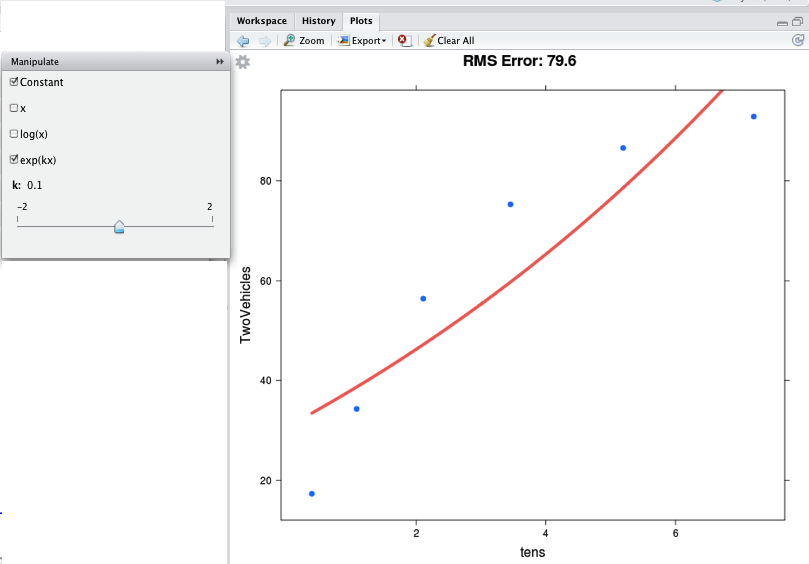
The check-boxes indicate which functions you want to take a linear combination of. You should check “Constant” and “exp(kx)”, as in the figure. Then you can use the slider to vary $k$ in order to make the function approximate the data as best you can. At the top of the graph is the RMS error — which here corresponds to the square root of the sum of square residuals. Making the RMS error as small as possible will give you the best $k$.

You may wonder, what was the point of the line that said

mutate(tens = Income / 10000)

This is just a concession to the imprecision of the slider. The slider works over a pretty small range of possible $k$, so this line constructs a new income variable with units of tens of thousands of dollars, rather than the original dollars. The instructions will tell you when you need to do such things.

5.2.1.1 Exercise 1

The data in "stan-data.csv" contains measurements made by Prof. Stan Wagon of the temperature of a cooling cup of hot water. The time was measured in seconds, which is not very convenient for the slider, so translate it to minutes. Then find the best value of $k$ in an exponential model.

water = read.csv("http://www.mosaic-web.org/go/datasets/stan-data.csv")
water$minutes = water$time/60
mFitExp( temp ~ minutes, data=water)

What’s the value of $k$ that gives the smallest RMS error? {-1.50,-1.25,-1.00,-0.75}
What are the units of this $k$? (This is not an R question, but a mathematical one.)
1. seconds
2. minutes
3. per second
4. per minute
Move the slider to set $k=0.00$. You will get an error message from the system about a “singular matrix.” This is because the function $e^{0x}$ is redundant with the constant function. What is it about $e^{kx}$ with $k=0$ that makes it redundant with the constant function?

5.2.1.2 Exercise 2

The "hawaii.csv" data set contains a record of ocean tide levels in Hawaii over a few days. The time variable is in hours, which is perfectly sensible, but you are going to rescale it to “quarter days” so that the slider will give better results. Then, you are going to use the mFitSines( ) program to allow you to explore what happens as you vary the nonlinear parameter $P$ in the linear combination $A \sin(\frac{2 \pi}{P} t) + B \cos(\frac{2 \pi}{P} t) + C$.

Hawaii = read.csv("http://www.mosaic-web.org/go/datasets/hawaii.csv")
Hawaii$quarterdays = Hawaii$time/6
mFitSines(water~quarterdays, data=Hawaii)

Check both the $\sin$ and $\cos$ checkbox, as well as the “constant.” Then vary the slider for $P$ to find the period that makes the RMS error as small as possible. Make sure the slider labeled $n$ stays at $n=1$. What is the period $P$ that makes the RMS error as small as possible (in terms of “quarter days”)?

3.95 quarter days
4.00 quarter days
4.05 quarter days
4.10 quarter days

You may notice that the “best fitting” sine wave is not particularly close to the data points. One reason for this is that the pattern is more complicated than a simple sine wave. You can get a better approximation by including additional sine functions with different periods. By moving the $n$ slider to $n=2$, you will include both the sine and cosine functions of period $P$ and of period $P/2$ — the “first harmonic.” Setting $n=2$ will give a markedly better match to the data.
What period $P$ shows up as best when you have $n=2$: {3.92,4.0,4.06,4.09,4.10,4.15}