24 Partial change

This is a good time to point out something we have been doing all along, but which has likely been such a persistent component of your mathematics education that you may not have realized that it is a construction. 2600

We have two ways by which we represent functions:

1. As a computational algorithm for generating the output from an input(s), typically involving arithmetic and such.
2. As a geometrical entity, specifically the graph of a function which can be a curve or, for functions of two inputs, a surface.

These two modes are sometimes intertwined, as when we use the name “line” to refer to a computational object: \(\line(x) \equiv a x + b\).

Unfortunately for functions of two inputs, a surface is hard to present in the formats that are most easily at hand: a piece of paper, a printed page, a computer screen. That’s because a curved surface is naturally a 3-dimensional object, while paper and screens provide two-dimensional images. Consequently, the graphics mode we prefer for presenting functions of two variables is the contour plot, which is not a single geometrical object but a set of many objects: contours, labels, colored tiles. 2605

We’ve been doing calculus on functions of one variable because it is so easy to exploit both the computational mode and the graphical mode. And it might fairly be taken as a basic organizing theme of calculus that 2610

a line segment approximates a curve in a small region around a point.

When figuring out the derivative function \(\partial_x f(x)\) from a graph of \(f(x)\), we find the tangent to the graph at each of many input values, record the slope of the line (and throw away the intercept) and then write down the series of slopes as a function of the input, typically by representing the slope by position along the vertical axis and the corresponding input by position along the horizontal axis. Figure 24.1 shows the process. 2615

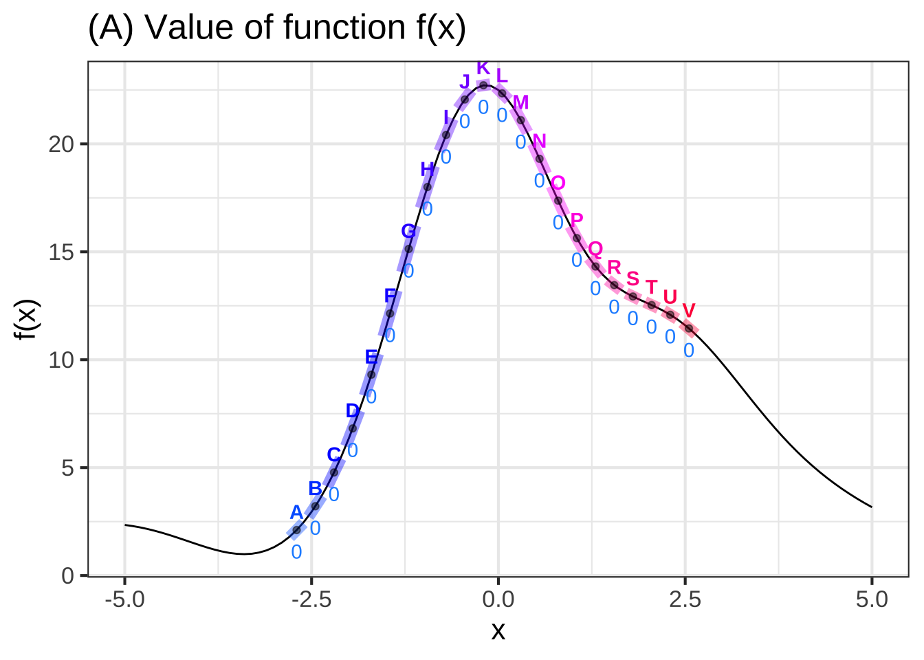
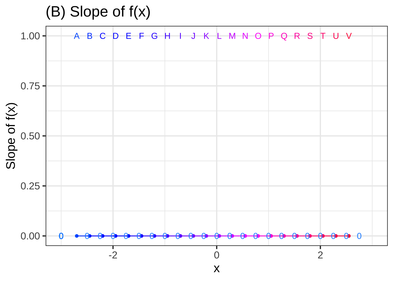
Figure 24.1: (A) The graph of a smooth function annotated with small line segments that approximate the function locally. The color of each labeled segment corresponds to the value of \(x\) for that segment. The slope of each segment is written numerically below the segment. (B) The labeled dots show the slope of each segment from (A). The slope is encoded using vertical position (as usual) and carries over the numerical label from (A). Connecting the dots sketches out the derivative of the function in (A).

Panel (A) in Figure 24.1 shows a smooth function \(f(x)\) (thin black curve). To find the function \(\partial_x f(x)\), we take the slope of \(f(x)\) at many closely spaced inputs. In Panel (A), we’ve highlighted short, tangent line segments at the closely-spaced points labeled A through V. The slope of each tangent line segment can be calculated by the usual rise-over-run method; the numerical value of the slope is written underneath the segment. To plot the derivative \(\partial_x f(x)\), I have taken the slope information from (A) and plotted it as a function of \(x\). 2620

To restate what you already know, in the neighborhood of any input value \(x\), the slope of any local straight-line approximation to \(f(x)\) is given by the value of of \(\partial_x f(x)\).

24.1 Calculus on two inputs

Although we use contour plots for good practical reasons, the graph of a function \(g(x,y)\) with two inputs is a surface, as described in Section 6.8. The derivative of \(g(x,y)\) should encode the information needed to approximate the surface at any input \((x,y)\). In particular, we want the derivative of \(g(x,y)\) to tell us the orientation of the tangent plane to the surface.

A tangent plane is infinite in extent. Let’s use the word facet to refer to a little patch of the tangent plane centered at the point of contact. Each facet is flat. (It’s part of a plane!) Figure 24.2 shows some facets tangent to a familiar curved surface. No two of the facets are oriented the same way.

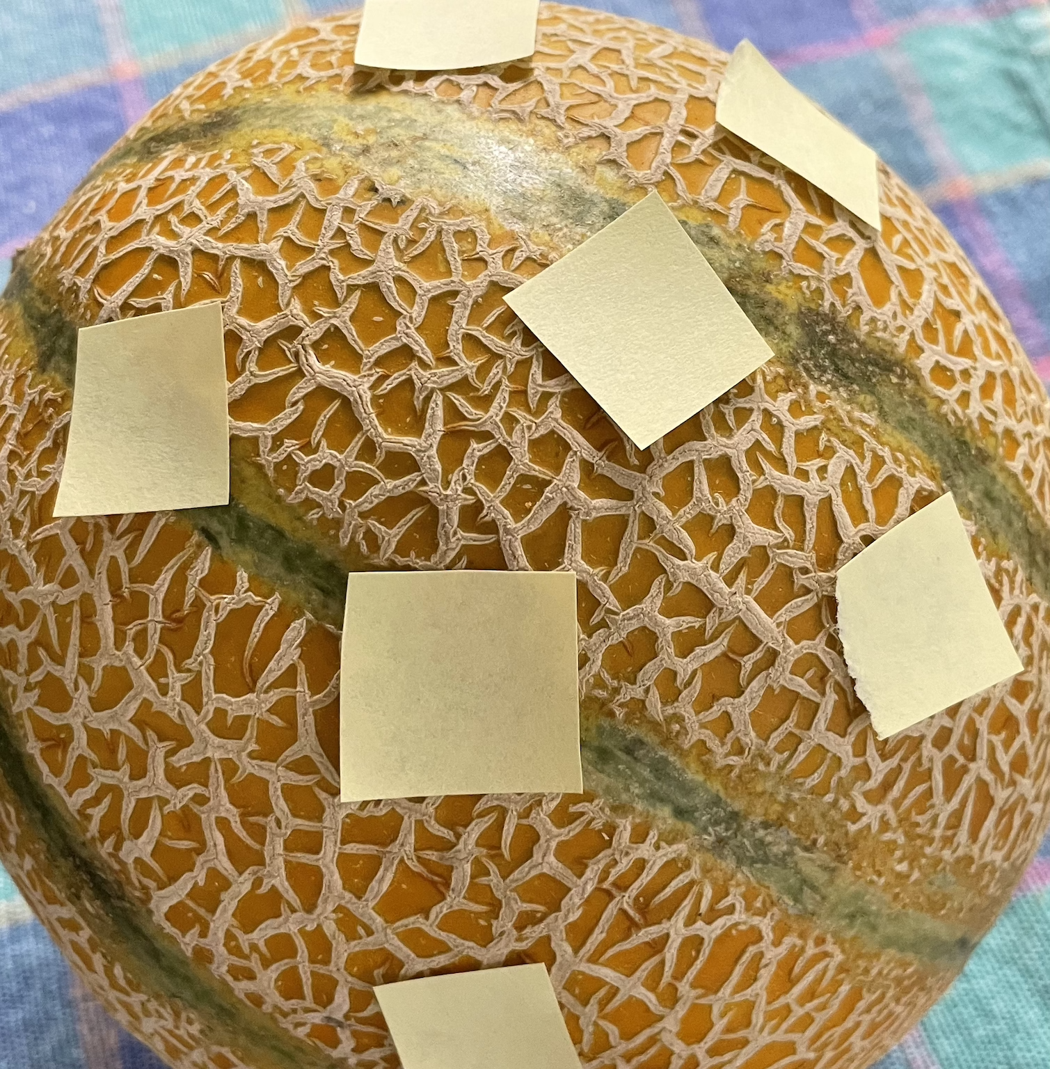
Figure 24.2: A melon as a model of a curved surface such as the graph of a function of two inputs. Each tangent facet has its own orientation. (Disregard the slight curvature of the small pieces of paper. Summer humidity has interfered with my attempt to model a flat facet with a piece of Post-It paper!

Better than a picture of a summer melon, pick up a hardcover book and place it on a curved surface such as a basketball. The book cover is a flat surface: a facet. The orientation of the cover will match the orientation of the surface at the point of tangency. Change the orientation of the cover and you will find that the point of tangency will change correspondingly. 2625

If melons and basketballs are not your style, you can play the same game on an interactive graph of a function of two variables. The snapshot below is a link to an applet that shows the graph of a function as a blue surface. You can specify a point on the surface by setting the value of the (x, y) input using the sliders. Display the tangent plane (which will be green) at that point by check-marking the “Tangent plane” input. (Acknowledgments to Alfredo Sánchez Alberca who wrote the applet using the GeoGebra math visualization system.) 2630

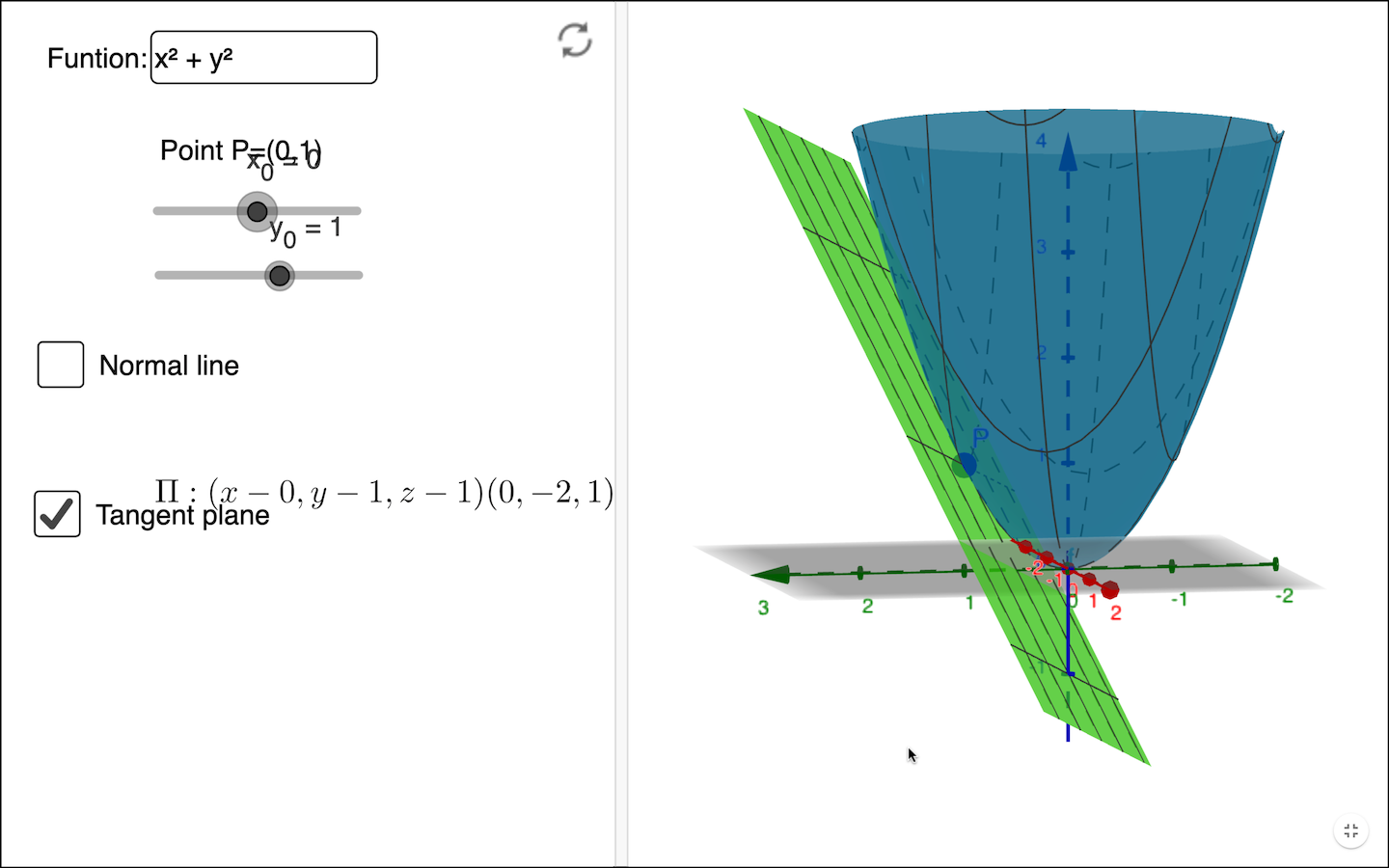
2635

For the purposes of computation by eye, a contour graph of a surface can be easier to deal with. Figure 24.3 shows the contour graph of a smoothly varying function. Three points have been labeled A, B, and C. 2640

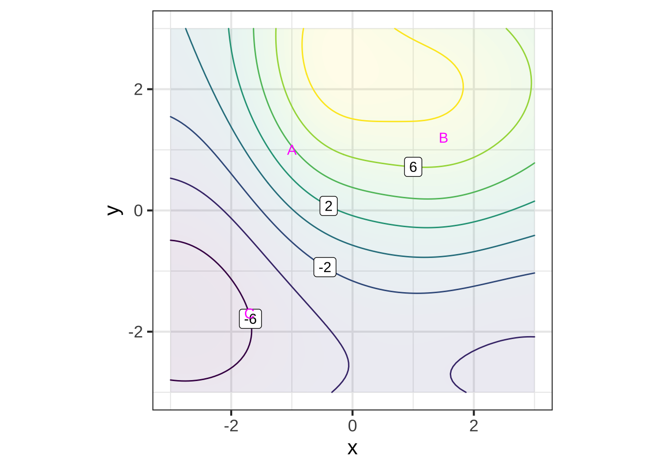
Figure 24.3: A function of 2 inputs with 3 specific inputs marked A, B, and C

Zooming in on each of the marked points presents a simpler picture for each of them, although one that is different for each point. Each zoomed-in plot contains almost parallel, almost evenly spaced contours. If the surface had been exactly planar over the entire zoomed-in domain, the contours would be exactly parallel and exactly evenly spaced. We can approach such exact parallelness by zooming in more closely around the labeled point. 2645

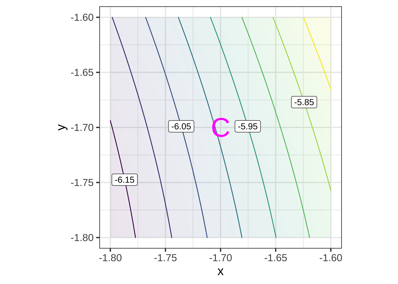
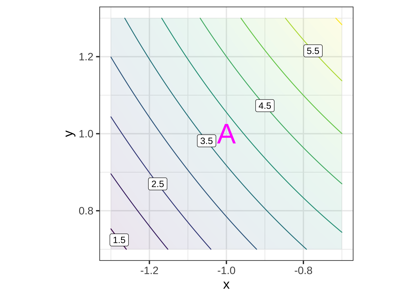
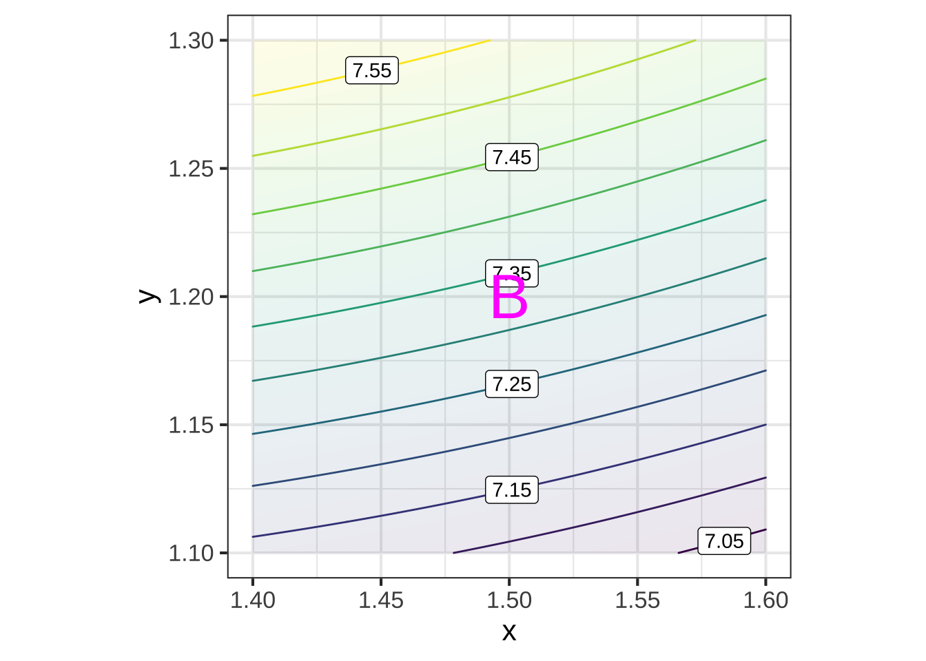
Figure 24.4: Zooming in on the neighborhoods of A, B, and C in Figure 24.3 shows a simple, almost planar, local landscape.

Just as the function \(\line(x) \equiv a x + b\) describes a straight line, the function \(\text{plane}(x, y) \equiv a + b x + c y\) describes a plane whose orientation is specified by the value of the parameters \(b\) and \(c\). (Parameter \(a\) is about the vertical location of the plane, not it’s orientation.) 2650

In Figure 24.5, the facets tangent to the original surface at A, B, and C are displayed. Comparing Figures 24.4 and 24.5 you can see that each facet has the same orientation as the surface; the contours face in the same way. 2655

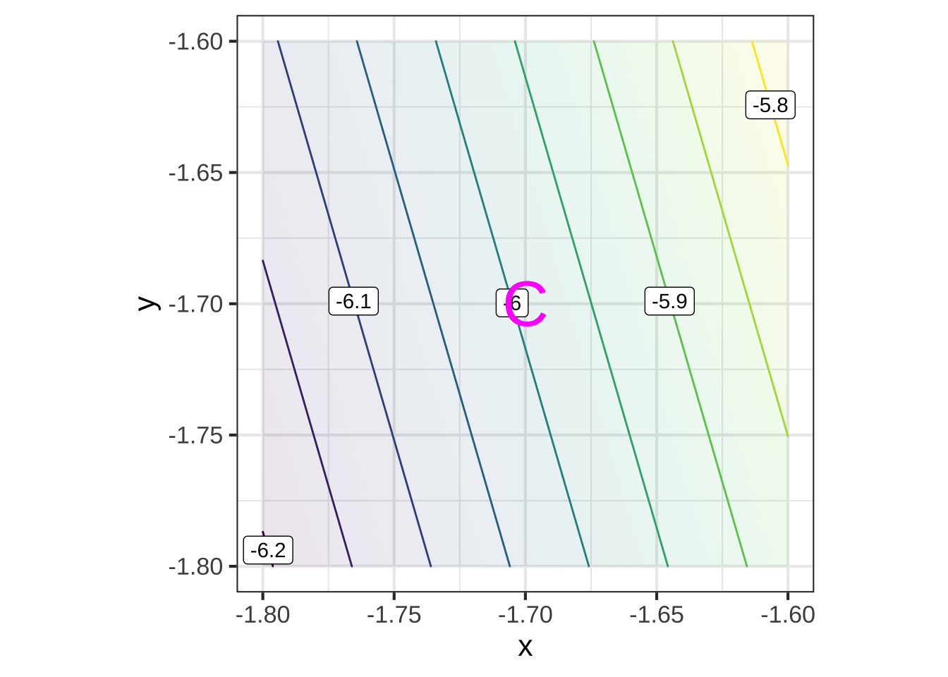
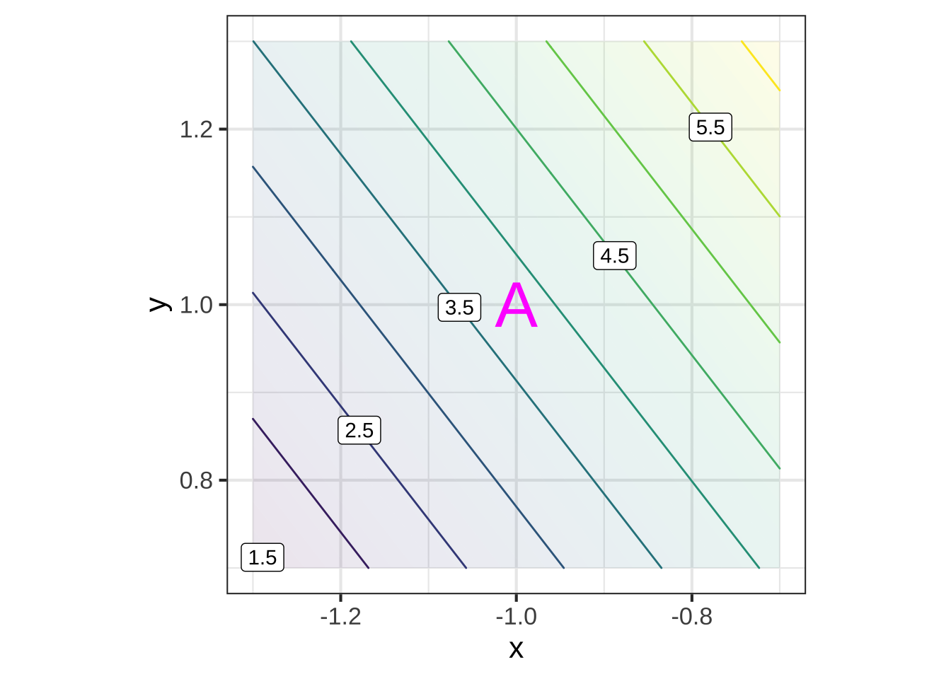
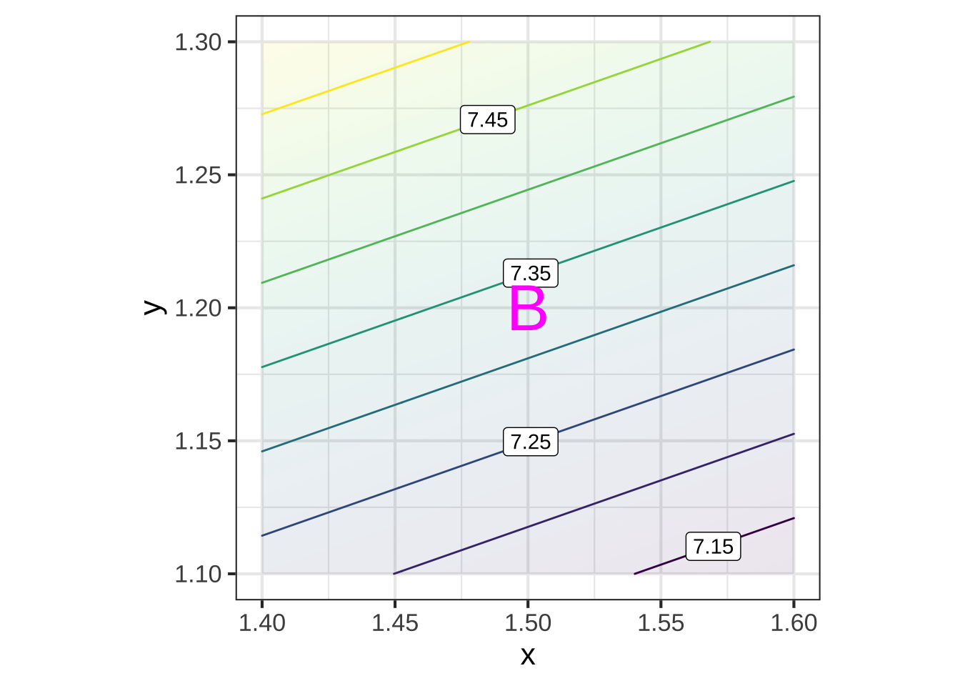
Figure 24.5: The facets around the points are linear functions, each aligned with the contours near that point in Figure 24.3

Remember that the point of constructing such facets is to generalize the idea of a derivative from a function of one input \(f(x)\) to functions of two or more inputs such as \(g(x,y)\). Just as the derivative \(\partial_x f(x_0)\) reflects the slope of the line tangent to the graph of \(f(x)\) at \(x=x_0\), our plan for the “derivative” of \(g(x_0,y_0)\) is to represent the orientation of the facet tangent to the graph of \(g(x,y)\) at \((x=x_0, y=y_0)\). The question for us now is what information is needed to specify an orientation. 2660

One clue comes from the formula for a function whose graph is a plane oriented in a particular direction:

\[\text{plane}(x,y) \equiv a + b x + cy\]

To explore the roles of the parameters \(b\) and \(c\) in setting the orientation of the line, open a SANDBOX. The scaffolding code generates a particular instance of \(\text{plane}(x,y)\) and plots it in two ways: a contour plot and a surface plot. Change the numerical values of \(b\) and \(c\) and observe how the orientation of the planar surface changes in the graphs. You can also see that the value of \(a\) is irrelevant to the orientation of the plane, just as the intercept of a straight-line graph is irrelevant to the slope of that line. 2665

plane <- makeFun(a + b*x + c*y ~ x + y, a = 1, b = -2.5, c = 1.6)
if (knitr::is_html_output()) {
  interactive_plot(plane(x, y) ~ x + y, domain(x=c(-2, 2), y=c(-2, 2)))
} else {
  knitr::include_graphics(normalizePath("www/plane-3d.png"))
}

contour_plot(plane(x, y) ~ x + y, domain(x=c(-2, 2), y=c(-2, 2))) %>%
  gf_refine(coord_fixed())

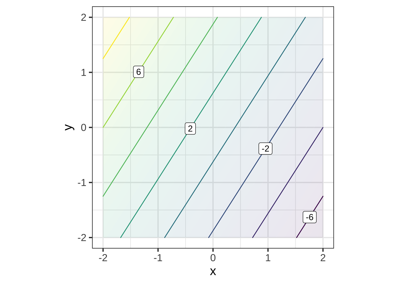As always it can be difficult to extract quantitative information from a surface plot. For the example here, you can see that the high-point on the surface is when \(x\) is most negative and \(y\) is most positive. Compare that to the contour plot to verify that that two modes are displaying the same surface. 2670

(Note: The gf_refine(coord_fixed()) part of the contour-plot command makes numerical intervals on the horizontal and vertical axes have the same length.)

An instructive experience is to pick up a rigid, flat object, for instance a smartphone or hardcover book. Hold the object level with pinched fingers at the mid-point of each of the short ends, as shown in Figure 24.6 (left). 2675

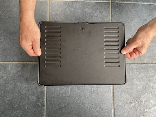
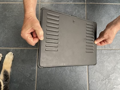
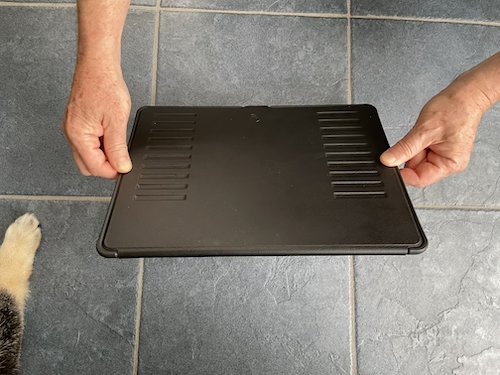
Figure 24.6: Combining two simple movements can tip a plane to all sorts of different orientations.

You can tip the object in one direction by raising or lowering one hand. (middle picture) And you can tip the object in the other coordinate direction by rotating the object around the line joining the points grasped by the left and right hands. (right picture) By combining these two motions, you can orient the surface of the object in a wide range of directions.³⁹ 2680

The purpose of this lesson is to show that two-numbers are sufficient to dictate the orientation of a plane. In terms of Figure 24.6 these are 1) the amount that one hand is raised relative to the other and 2) the angle of rotation around the hand-to-hand axis. 2685

Similarly, in the formula for a plane, the orientation is set by two numbers, \(b\) and \(c\) in \(\text{plane}(x, y) \equiv a + b x + c y\).

How do we find the right \(b\) and \(c\) for the tangent facet to a function \(g(x,y)\) at a specific input \((x_0, y_0)\)? Taking slices of \(g(x,y)\) provides the answer. In particular, these two slices: \[\text{slice}_1(x) \equiv g(x, y_0) = a + b\, x + c\, y_0 \\ \text{slice}_2(y) \equiv g(x_0, y) = a + b x_0 + c\, y\]

Look carefully at the formulas for the slices. In \(\text{slice}_1(x)\), the value of \(y\) is being held constant at \(y=y_0\). Similarly, in \(\text{slice}_2(y)\) the value of \(x\) is held constant at \(x=x_0\). 2690

The parameters \(b\) and \(c\) can be read out from the derivatives of the respective slices: \(b\) is equal to the derivative of the slice\(_1\) function with respect to \(x\) evaluated at \(x=x_0\), while \(c\) is the derivative of the slice\(_2\) function with respect to \(y\) evaluated at \(y=y_0\). Or, in the more compact mathematical notation:

\[b = \partial_x \text{slice}_1(x)\left.\strut\right|_{x=x_0} \ \ \text{and}\ \ c=\partial_y \text{slice}_2(y)\left.\strut\right|_{y=y_0}\] These derivatives of slice functions are called partial derivatives. The word “partial” refers to examining just one input at a time. In the above formulas, the \({\large |}_{x=x_0}\) means to evaluate the derivative at \(x=x_0\) and \({\large |}_{y=y_0}\) means something similar. 2695

You don’t need to create the slices explicitly in order to calculate the partial derivatives. Simply differentiate \(g(x, y)\) with respect to \(x\) in order to get parameter \(b\) and differentiate \(g(x, y)\) with respect to \(y\) to get parameter \(c\). To demonstrate, we’ll make use of the sum rule: \[\partial_x g(x, y) = \underbrace{\partial_x a}_{=0} + \underbrace{\partial_x b x}_{=b} + \underbrace{\partial_x cy}_{=0} = b\] Similarly, \[\partial_y g(x, y) = \underbrace{\partial_y a}_{=0} + \underbrace{\partial_y b x}_{=0} + \underbrace{\partial_y cy}_{=c} = c\]

Get in the habit of noticing the subscript on the differentiation symbol \(\partial\). When taking, for instance, \(\partial_y f(x,y,z, \ldots)\), all variables other than \(y\) are to be held constant. Some examples: 2700

\[\partial_y 3 x^2 = 0\ \ \text{but}\ \ \ \partial_x 3 x^2 = 6x\\ \ \\ \partial_y 2 x^2 y = 2x^2\ \ \text{but}\ \ \ \partial_x 2 x^2 y = 4 x y \]

24.2 All other things being equal …

Recall that the derivative of a function of one variable, say, \(\partial_x f(x)\) tells you, at each possible value of the input \(x\), how much the output will change proportional to a small change in the value of the input.

Now that we are in the domain of multiple inputs, writing \(h\) to stand for “a small change” is not entirely adequate. Instead, we’ll write \(dx\) for a small change in the \(x\) input and \(dy\) for a small change in the \(y\) input.

With this notation, we write the first-order polynomial approximation to a function of a single input \(x\) as \[f(x+dx) = f(x) + \partial_x f(x) \times dx\] Applying this notation to functions of two inputs, we have: \[g(x + \color{magenta}{dx}, y) = g(x,y) + \color{magenta}{\partial_x} g(x,y) \times \color{magenta}{dx}\\ \text{and} \\ g(x, y+\color{brown}{dy}) = g(x,y) + \color{brown}{\partial_y} g(x,y) \times \color{brown}{dy}\]

Each of these statements is about changing one input while holding the other input(s) constant. Or, as the more familiar expression goes, "The effect of changing one input all other things being equal or all other things held constant.⁴⁰ 2705

Everything we’ve said about differentiation rules applies not just to functions of one input, \(f(x)\), but to functions with two or more inputs, \(g(x,y)\), \(h(x,y,z)\) and so on. 2710

24.3 Gradient vector

For functions of two inputs, there are two partial derivatives. For functions of three inputs, there are three partial derivatives. We can, of course, collect the partial derivatives into Cartesian coordinate form. This collection is called the gradient vector. 2715

Just as our notation for differences (\(\cal D\)) and derivatives (\(\partial\)) involves unusual typography on the letter “D,” the notation for the gradient involves such unusual typography although this time on \(\Delta\), the Greek version of “D.” For the gradient symbol, turn \(\Delta\) on its head: \(\nabla\). That is, \[\nabla g(x,y) \equiv \left(\stackrel\strut\strut\delta_x g(x,y), \ \ \delta_y g(x,y)\right)\]

Note that \(\nabla g(x,y)\) is a function of both \(x\) and \(y\), so in general the gradient vector differs from place to place in the function’s domain.

The graphics convention for drawing a gradient vector for a particular input, that is, \(\nabla g(x_0, y_0)\), puts an arrow with its root at \((x_0, y_0)\), pointing in direction \(\nabla g(x_0, y_0)\), as in Figure 24.7. 2720

Figure 24.7: The gradient vector \(\nabla g(x=1,y=2)\). The vector points in the steepest uphill direction. Consequently, it is perpendicular to the contour passing through its root.

A gradient field (see Figure 24.8) is the value of the gradient vector at each point in the function’s domain. Graphically, in order to prevent over-crowding, the vectors are drawn at discrete points. The lengths of the drawn vectors are set proportional to the numerical length of \(\nabla g(x, y)\), so a short vector means the surface is relatively level, a long vector means the surface is relatively steep. 2725

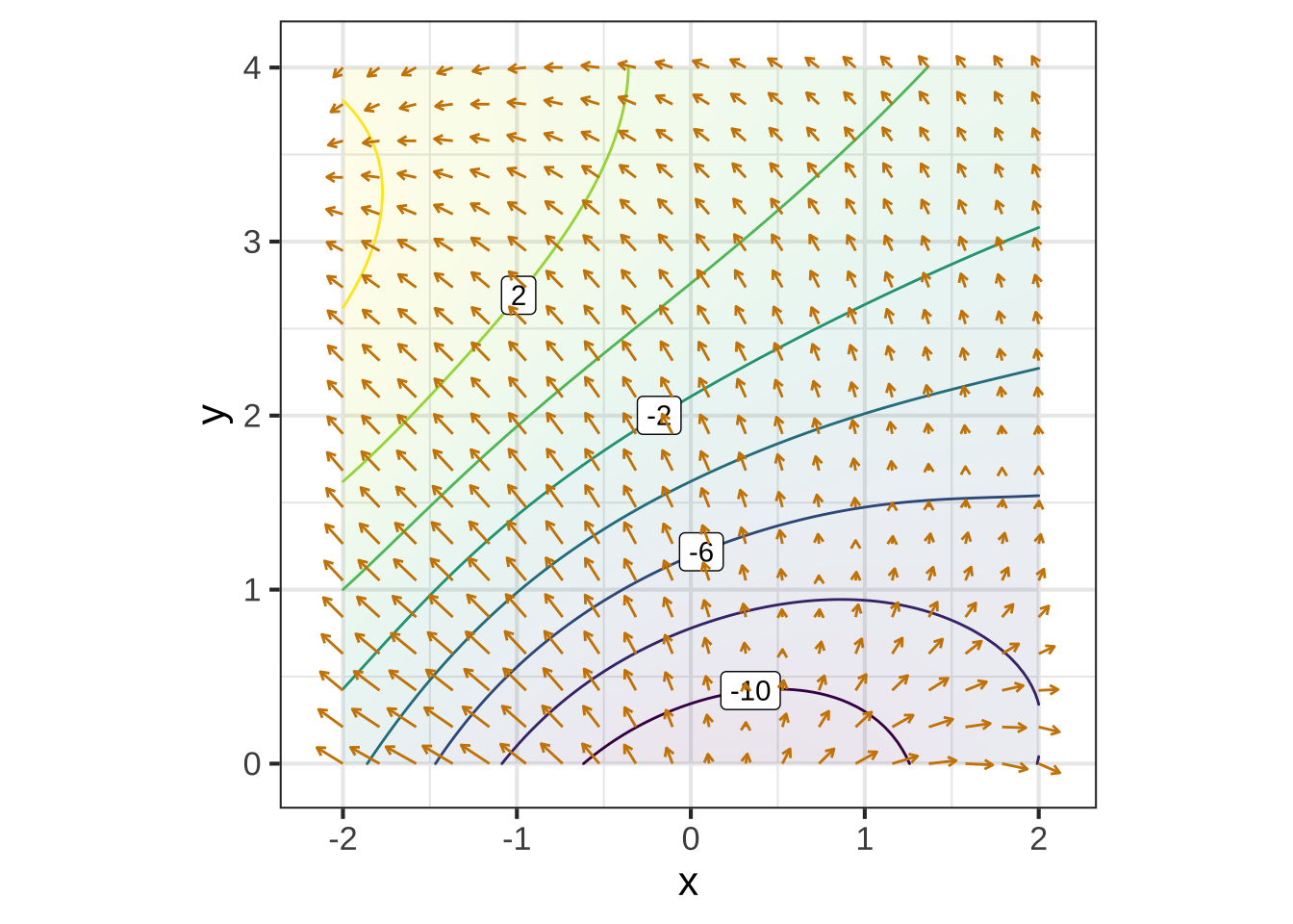
Figure 24.8: A plot of the gradient field \(\nabla g(x,y)\).

24.4 Total derivative (optional)

The name “partial derivative” suggests the existence of some kind of derivative that’s not just a part, but the whole thing. The total derivative is such a whole and gratifyingly made up of it’s parts, that is, the partial derivatives.

Suppose you are modeling the temperature of some volume of the atmosphere, given as \(T(t, x, y, z)\). This merely says that the temperature depends on both time and location, something that is familiar from everyday life.

The partial derivatives have an easy interpretation: \(\partial_t T()\) tells how the temperature is changing over time at a given location, perhaps because of the evaporation or condensation of water vapor. \(\partial_x T()\) tells how the temperature changes in the \(x\) direction, and so on.

The total derivative gives an overall picture of the changes in a parcel of air, which you can thnk of as a tiny balloon-like structure but without the balloon membrane. The temperature inside the “balloon” may change with time (e.g. condensation or evaporation of water), but as the ballon drifts along with the motion of the air (that is, the wind), the evolving location can change the temperature as well. Think of a balloon caught in an updraft: the temperature goes down as the balloon ascends.

For an imaginary observer located in the balloon, the temperature is changing with time. Part of this change is the instrinsic change measured by \(\partial_t T\) but we need to add to that the changes induces by the evolving location of the balloon. The partial change in temperature due to a change in altitude is \(\partial_z T\), but it’s important to realize that the coordinates of the location are themselves functions of time: \(x(t), y(t), z(t)\). Seeing the function \(T()\) for the observer in the balloon as a function of \(t\), we have \(T(t, x(t), y(t), z(t))\). This is a function composition: \(T()\) composed with each of \(x()\), \(y()\), and \(z()\). Recall in the chain rule \(\partial_v f(g(v)) = \partial_v f(g(v)) \partial_v g(v)\) that the derivative of the composed quantity is the product of two derivatives.

Likewise, the total derivative of temperature with respect to the observer riding in the balloon will be add together the parts due to changes in time (holding position constant), x-coordinate (holding time and the other space coordinates constant), and the like. Signifying the total differentiation with a capital \(D\), we have \[D\, T(t) = \partial_t T() + \partial_x T() \cdot\partial_t x + \partial_y T()\cdot \partial_t y + \partial_z T() \cdot\partial_t z\] Note that \(\partial_t x\) is the velocity of the balloon in the x-direction, and similarly for the other coordinate directions. Writing these velocities as \(v_x, v_y, v_z\), the total derivative for temperature of a parcel of air embedded in a moving atmosphere is

\[D\ T(t) = \partial_t T + v_x\, \partial_x T + v_y\, \partial_y T + v_z\, \partial_z T\] Formulations like this, which put the parts of change together into a whole, are often seen in the mathematics of fluid flow as applied in meteorology and oceanology.

24.5 Differentials

A little bit of this, a little bit of that. — Stevie Wonder, “The Game of Love”

We have framed calculus in terms of functions: transformations that take one (or more!) quantities as input and return a quantity as output. This was not the original formulation. In this section, we will use the original style in order to demonstrate how you can sometimes skip the step of constructing a function before differentiating to answer a question of the sort: “If this quantity changes by a little bit, how much will another, related quantity change?”

As an example, consider the textbook-style problem of a water skier being pulled along the water by a rope pulled in from the top of a tower of height \(H\). The skier is distance \(x\) from the tower. As the rope is winched in at a constant rate, does the skier go faster or slower as she approaches the tower.

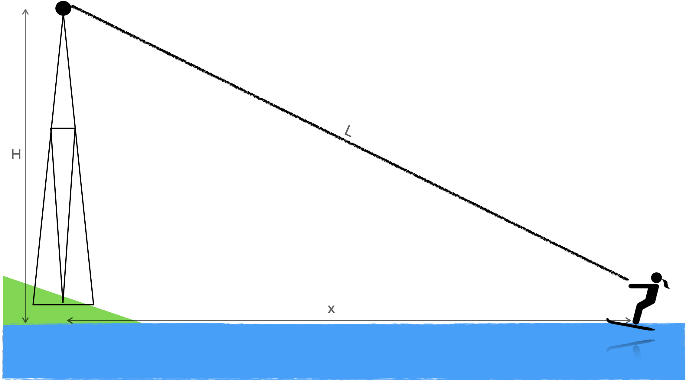
In the function style of approach, we can write the position function \(x(t)\) with input the length of the rope \(L(t)\). Using the diagram, you can see that \[x(t) = \sqrt{\strut L(t)^2 - H^2}\ .\]

Differentiate both sides with respect to \(t\) to get the velocity of the skier: \(\partial_t x(t)\) through the chain rule: \[\underbrace{\partial_t x(t)}_{\partial_t f(g(t))} = \underbrace{\frac{1}{2\sqrt{\strut L(t)^2 - H^2}}}_{\left[ \partial_t f \right](g(t)) } \times \underbrace{\left[2 \partial_t L(t)\right]}_{\partial_t g(t)} = \frac{\partial_t L(t)}{\strut\sqrt{L(t)^2 - H^2}}\]

Now to reformulate the problem without defining a function.

Newton referred to “flowing quantities” or “fluents” and to what today is universally called derivatives as “fluxions.” Newton did not have a notion of inputs and output.⁴¹

At about the same time as Newton’s inventions, very similar ideas were being given very different names by mathematicians on the European continent. There, an infinitely small change in a quantity was called a “differential” and the differential of \(x\) was denoted \(dx\).

The first calculus textbook was subtitled, Of the Calculus of Differentials, in other words, how to calculate differentials. (See Figure 24.9.) Section I of this 1696 text is entitled, “Where we give the rules of this calculation,” those rules being recognizably the same as presented in Chapter 22 of this book.

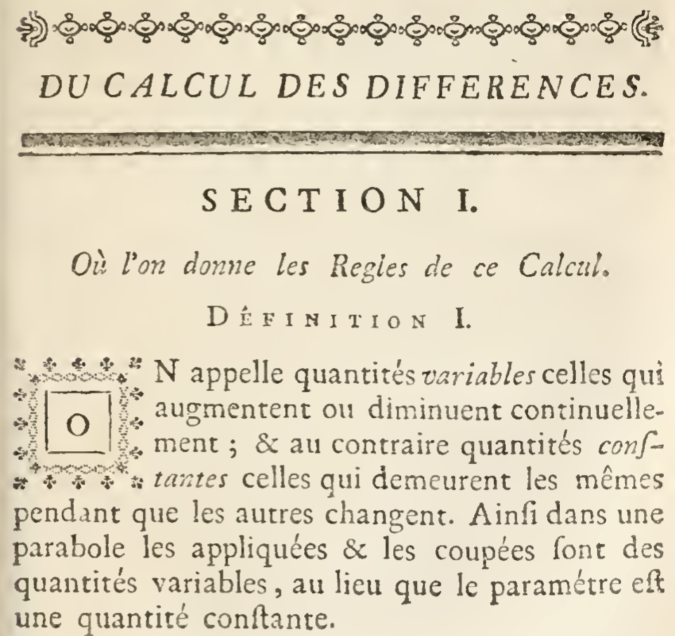
Figure 24.9: From the start of the first calculus textbook, by le marquis de l’Hôpital, 1696.

Definition I of Section I states,

"We call quantities variable* that grow or decrease continuously; and to the contrary constant quantities are those that remain the same while the others change. … The infinitely small amount by which a continuous quantity increases or decreases is called the differential.*"

The differential is not a derivative. The differential is an infinitely small change in a quantity and a derivative is a rate of change. The differential of a quantity \(x\) is written \(dx\) in the textbook.⁴²

The point of Section I of de l’Hôpital’s textbook is to present the rules by which the differentials of complex quantities can be calculated. You’ll recognize the product rule in de l’Hôpital’s notation:

Figure 24.10: The differential of \(x\,y\) is \(y\,dx + x\,dy\)

The Pythagorean theorem relates the various quantities this way:

\[L^2 = x^2 + H^2\]

The differential of each side of the equation refers to “a little bit” of increase in the quantity on that side of the equation: \[d(L^2) = d(x^2)\ \ \ \implies\ \ \ 2 L\, dL = 2 x\, dx\] where we’ve used one of the “rules” for calculating differentials. This gives us \[dx = \frac{L}{x} dL\] Think of this as a recipe for calculating \(dx\). If you tell me \(L\), \(x\), and \(dL\) then you can calculate the value of \(dx\). For instance, suppose the tower is 52 feet tall and that there is \(L=173\) feet of tow-rope extending to the skier. The Pythagorean theorem tells us the skier is \(x=165\) feet from the base of the tower. The rope is, let us suppose, being pulled in at the top of the tower at \(dL = 10\) feet per second. How fast is \(x\) changing? \[dx = \frac{173\ \text{ft}}{165\ \text{ft}} \times 10 \text{ft s}^{-2} = 10.05\ \text{ft s}^{-1}\]

We’ll return to “a little bit of this” when we explore how to add up little bits to get the whole in Chapter 31.

24.6 Exercises

Exercise 24.01: xdkw

It’s relatively easy to assess partial derivatives when you know the gradient. After all, the gradient is the vector of \((\partial_x\,f(x,y), \partial_y f(x,y))\). To train your eye, here’s a contour plot and a corresponding gradient plot.

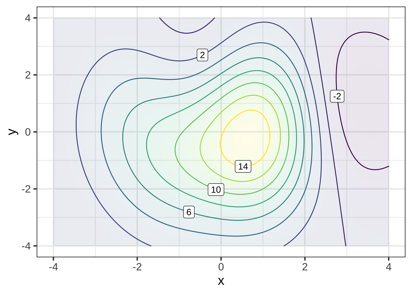
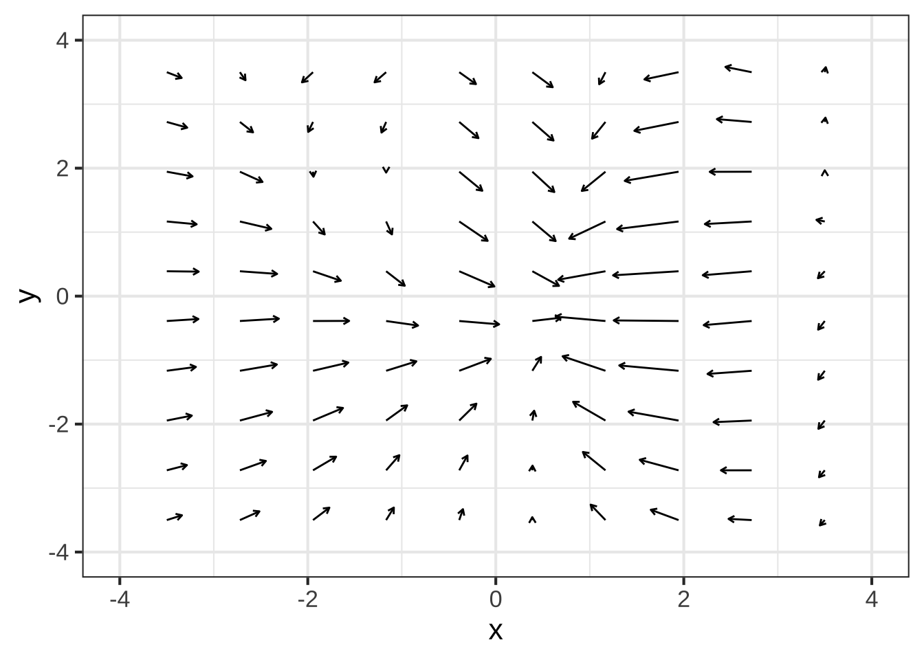
What is the rule for determining $$\partial_x f(x,y)$$ from the direction of the gradient vector? 



(x )  If the vector has a component pointing right, $$\partial_x f$$ is positive.
( )  If the vector has a component pointing left, $$\partial_x f$$ is positive
( )  If the vector has a vertical component pointing up, $$\partial_x f$$ is positive.
( )  If the vector has a component pointing downward, the partial derivative $$\partial_x f$$ is positive.

[[Right!]]

What is the rule for determining $$\partial_y f(x,y)$$ from the direction of the gradient vector? 



( )  If the vector has a component pointing right, $$\partial_y f$$ is positive.
( )  If the vector has a component pointing left, $$\partial_y f$$ is positive.
(x )  If the vector has a vertical component pointing up, $$\partial_y f$$ is positive.
( )  If the vector has a component pointing downward, the partial derivative $$\partial_y f$$ is positive.

[[Right!]]

Exercise 24.02: 9iowVB

Open a sandbox and use the following commands to make a contour plot of the function \(g(x)\) centered on the reference point \((x_0\!=\!0,\, y_0\!=\!0)\).

g <- rfun( ~ x + y, seed = 802, n = 15)
x0 <-  0
y0 <-  0
size <- 5
contour_plot(g(x, y) ~ x + y,
             domain(x = x0 + size*c(-1, 1),
                    y = y0 + size*c(-1, 1)))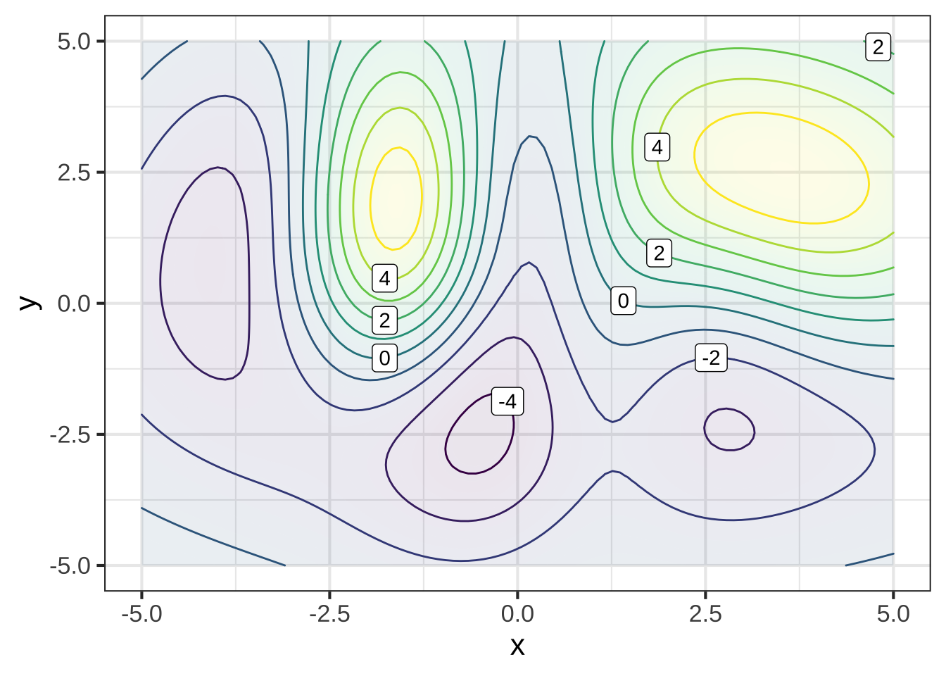 

By making size smaller, you can zoom in around the reference point. Zoom in gradually (say, size = 1.0, 0.5, 0.1, 0.05, 0.01) until you reach a point where the surface plot is (practically) a pretty simple inclined plane.

From the contour plot, zoomed in so that the graph shows an inclined plane, figure out the sign of \(\partial_x g(0,0)\) and \(\partial_y g(0,0)\).

Which answer best describes the signs of the partial derivatives of $$g(x,y)$$ at the reference point $$(x_0=0, y_0=0)$$?  



( )  $$\partial_x g(0,0)$$ is pos, $$\partial_y g(0,0)$$ is pos 
( )  $$\partial_x g(0,0)$$ is pos, $$\partial_y g(0,0)$$ is neg 
( )  $$\partial_x g(0,0)$$ is neg, $$\partial_y g(0,0)$$ is neg 
(x )  $$\partial_x g(0,0)$$ is neg, $$\partial_y g(0,0)$$ is pos.
( )  $$\partial_x g(0,0)$$ is 0, $$\partial_y g(0,0)$$ is pos

[[Good.]]

Exercise 24.04: qdkw

Consider this close up of a function around a reference point at the center of the graph.

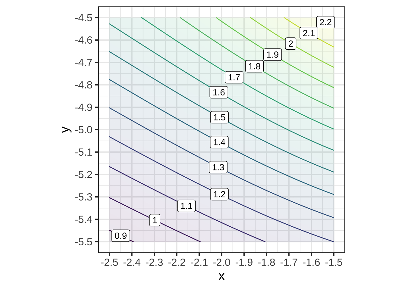
By eye, estimate these derivatives of the function at the reference point \((x_0=-2, y_0=-5)\).

What is the numerical value  of $$\partial_x g(x,y)$$ at the reference point? 



( )  -1
( )  -0.50
( )  -0.25
( )  0
( )  0.25
(x )  0.50
( )  1

[[Good.]]

What is the numerical value  of $$\partial_y g(x,y)$$ at the reference point? 



( )  -1
( )  -0.50
( )  -0.25
( )  0
( )  0.25
( )  0.50
(x )  1

[[Excellent!]]

The next questions ask about second-order partial derivatives. As you know, the second derivative is about how the first derivative changes with x or y. Insofar as the function is a simple inclined plane, where the contours would be straight, parallel, and evenly spaced, the second derivatives would all be zero. But you can see that it is not such a plane: the contours curve a bit.

In determining the second derivatives by eye from the graph, you are encouraged to compare first derivatives at the opposing edges of the graph, as opposed to at very nearby points.

What is the sign  of $$\partial_{xx} g(x,y)$$ at the reference point? 



(x )  negative
( )  positive

[[Excellent!]]

What is the sign  of $$\partial_{yy} g(x,y)$$ at the reference point? 



( )  negative
(x )  positive

[[Correct.]]

What is the sign  of $$\partial_{xy} g(x,y)$$ at the reference point? 



( )  negative
(x )  positive

[[Good.]]

What is the sign  of $$\partial_{yx} g(x,y)$$ at the reference point? 



( )  negative
(x )  positive

[[Right!]]

Exercise 24.06: uekses

At numerous occasions in your professional life, you will be in one or both of these positions:

1. You are a decision-maker being presented with the results of analysis conducted by a team of unknown reliability, and you need to figure out whether what they are telling you is credible.
2. You are a member of the analysis team needing to demonstrate to the decision-maker that your work should be believed.

As an example, consider one of the functions presented in a comedy book, Geek Logic: 50 Foolproof Equations for Everyday Life (2006), by Garth Sundem. The particular function we’ll consider here is Dr(), intended to help answer the question, “Should you go to the doctor?”

\[\text{Dr}(d, c, p, e, n, s) = \frac{\frac{s^2}{2} + e(n-e)}{100 - 3(d + \frac{p^3}{70} - c)}\] where

• \(d\) = How many days in the past month have you been incapacitated? \(d_0 \equiv 3\)
• \(c\) = Does the issue seem to be getting better or worse. (-10 to 10 with -10 being “circling the drain” and 10 being “dramatic improvement”) \(c_0 \equiv -2\)
• \(p\) = How much pain or discomfort are you currently experiencing? (1-10 with 10 being “currently holding detached toe in Ziploc bag”) \(p_0 = 3\)
• \(e\) = How embarrassing is this issue? (1-10 with 10 being “slipped on ice and fell on 1972 Mercedes-Benz hood ornament, which is now part of my body”) \(e_0 = 4\)
• \(n\) = How noticeable is the issue? (1-10 with 10 being “fell asleep on waffle iron”) \(n_0 = 5\)
• \(s\) = How serious does the issue seem? (1-10 with 10 being “may well have nail embedded in frontal lobe [of brain]”) \(s_0 = 3\)

Although the function is offered tongue-in-cheek, let’s examine it to see if it even roughly matches common sense. The tool we will use relates to low-order polynomial approximation around a reference point and examining appropriate partial derivatives. To save time, we stipulate a reference point for you, noted in the description of variables above.

The code creates an R implementation of the function that is set up so that the default values of the variables are those at the given reference point. You can use this in a sandbox to try different changes in each of the input quantities.

Dr <- makeFun(
  ((s^2)/2 + e*(n-e)) /
    (100 - 3*(d + (p^3/70) - c)) ~
    d+p+e+c+n+s, s=3, n=5, e=4, p=3, d=3, c=-2)
Dr()

According to the instructions in the book, if Dr()\(> 1\), you should go to the doctor.

Essay 1: The value of Dr() at the reference point is 0.10, indicating that you shouldn’t go to the doctor. But we don’t yet know whether 0.10 is very close to the decision threshold of 1 or very far away. Describe a reasonable way to figure this out. Report your description and the results here.

Essay 2: There are six inputs to the function. Go through the list of all six and (without thinking too hard about it) write down for all of them your intuitive sense of whether an increase of one point in that input should raise or lower the output of Dr() at the reference point. Also write down whether you think the input should be a large or small determinant of whether to go to the doctor. (You don’t need to refer to the Dr() function itself, just to your own intuitive sense of what should be the effect of each of the inputs.)

The operator D() can calculate partial derivatives. You can calculate the value of a partial derivative very easily at the reference point, using an expression like this, which gives the value of the partial of Dr() with respect to input \(s\) at the reference point:

D(Dr(s = s) ~ s)(s=3)

We’re now going to use these partial derivatives to compare your intuition about going to the doctor to what the function has to say. Of course, we don’t know yet whether the function is reasonable, so don’t be disappointed if your intuition conflicts with the function.

Essay 3: Calculate the numerical value of each of the partial derivatives at the reference point. List them here and say, for each one, whether it accords with your intuition.

Exercise 24.07: RbuhMy

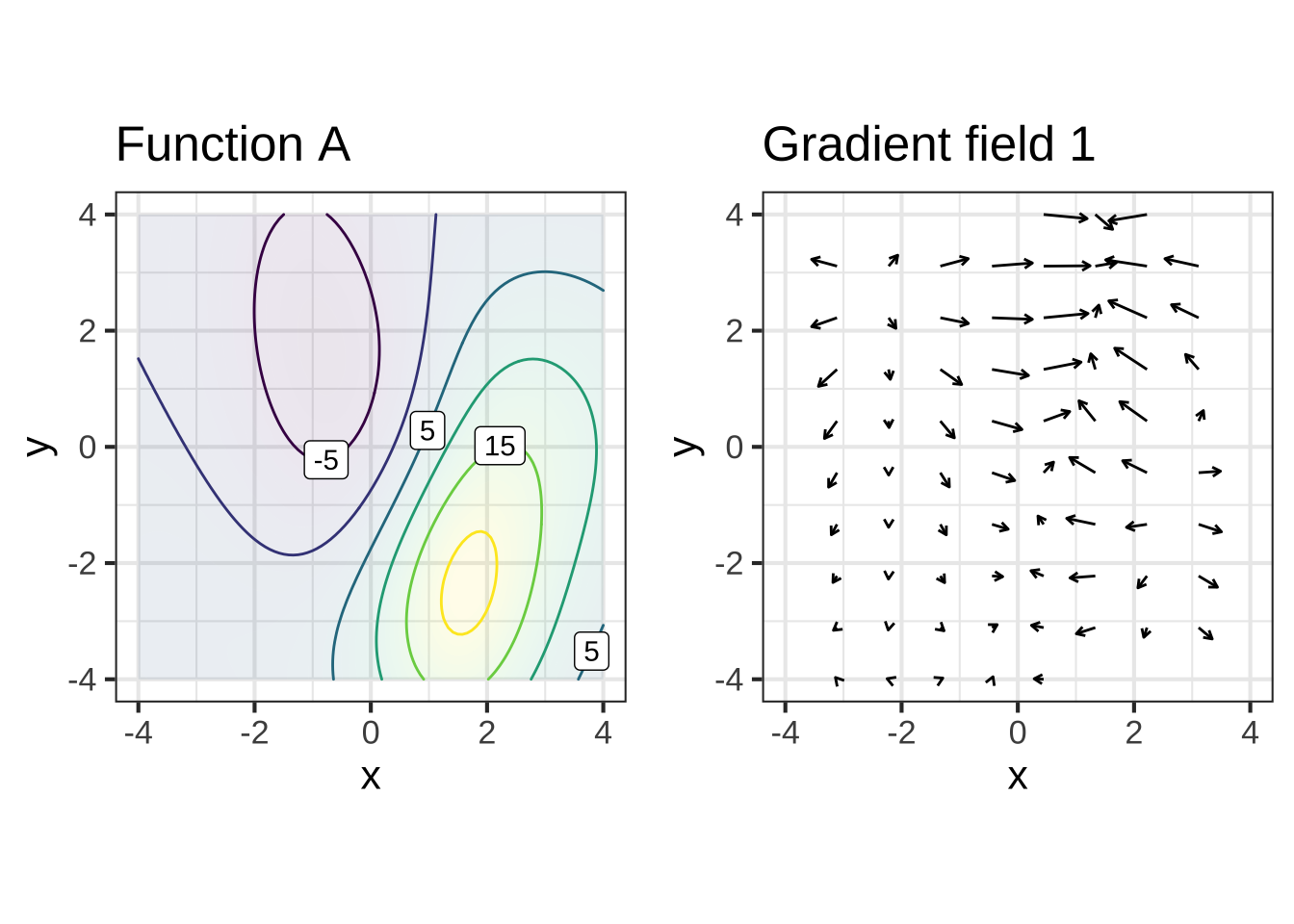
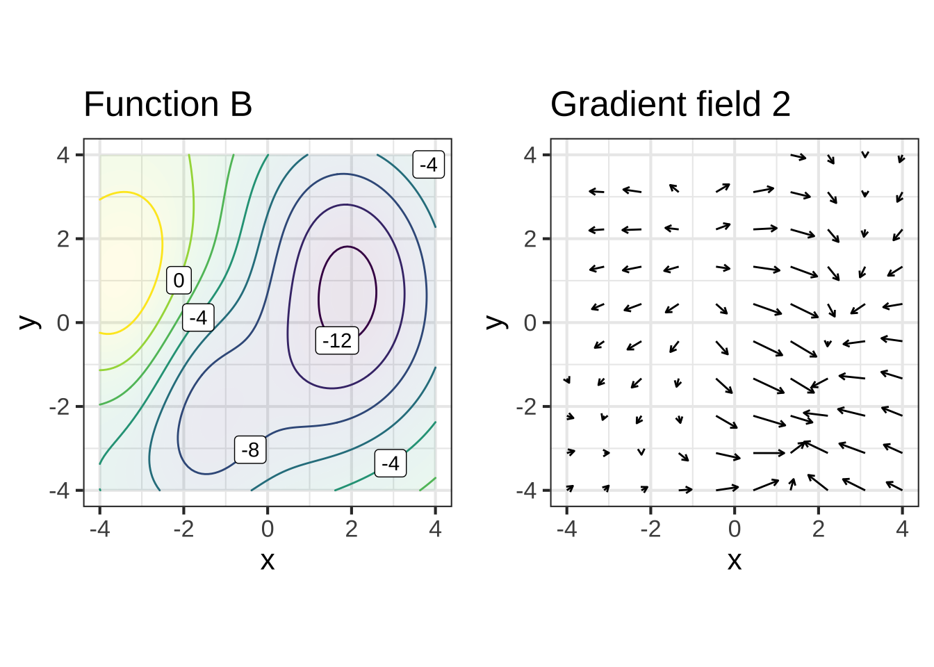
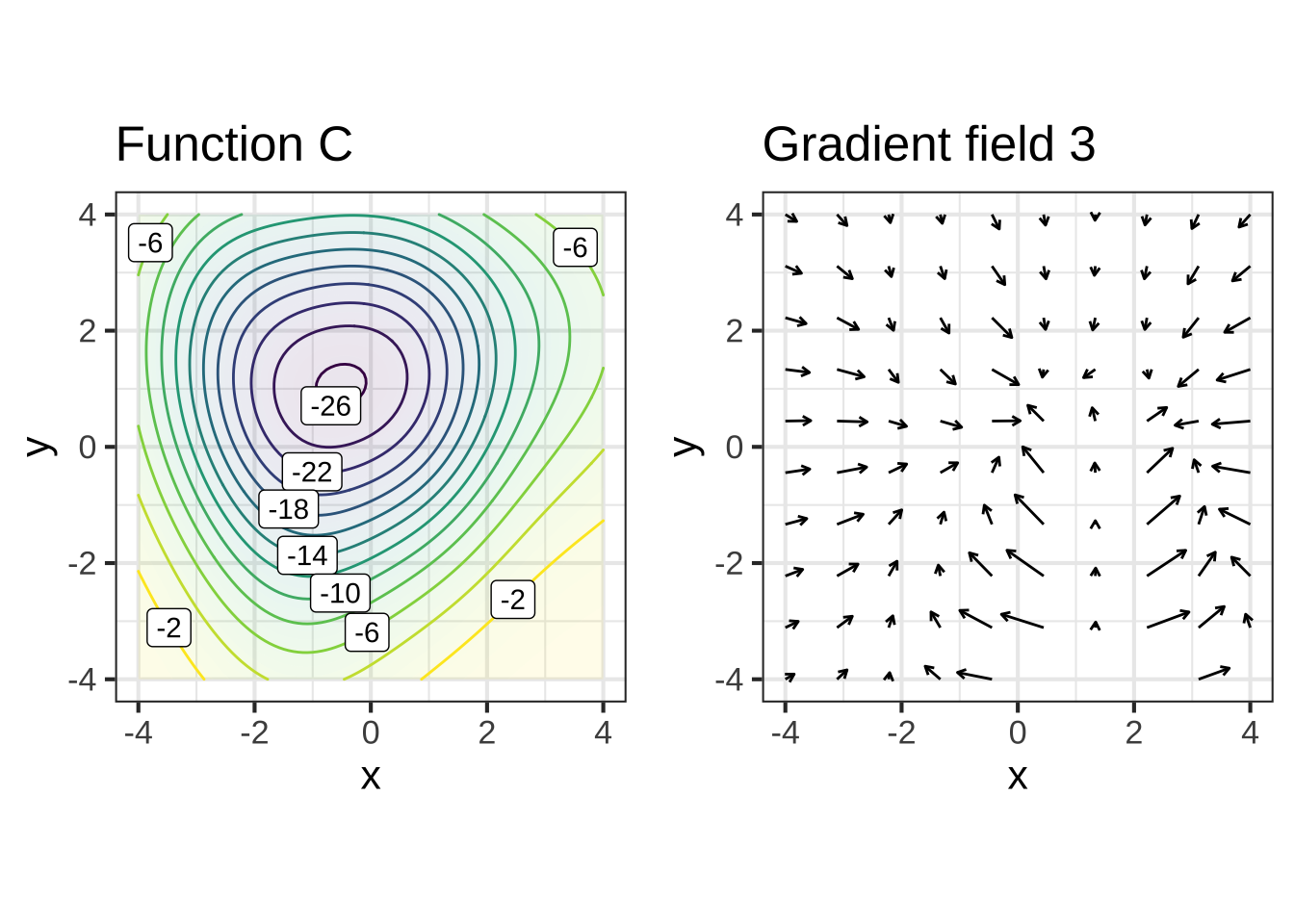
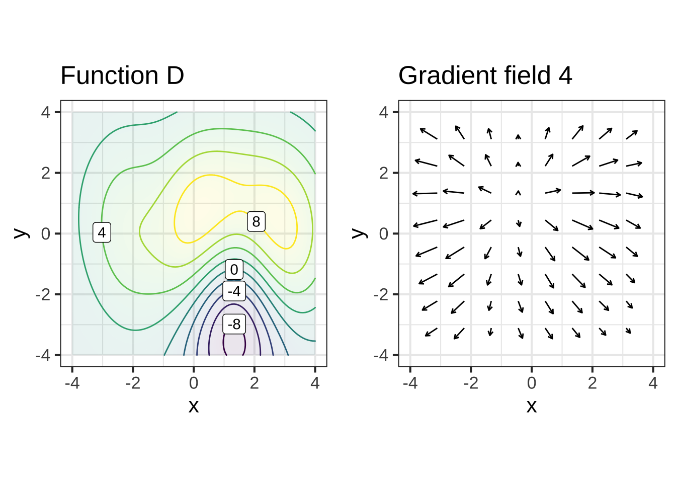
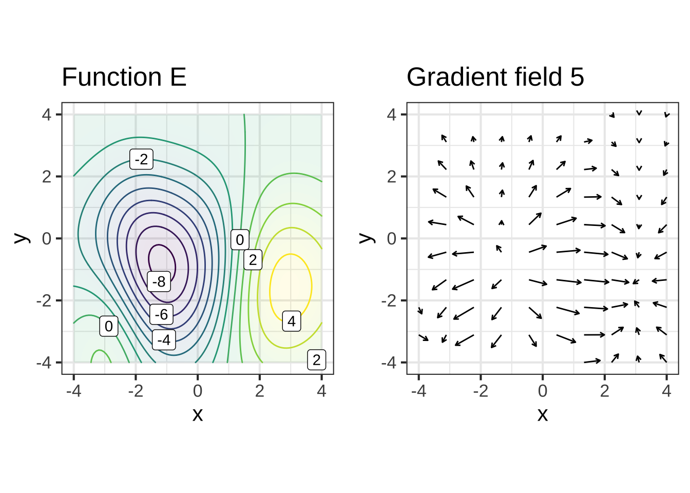
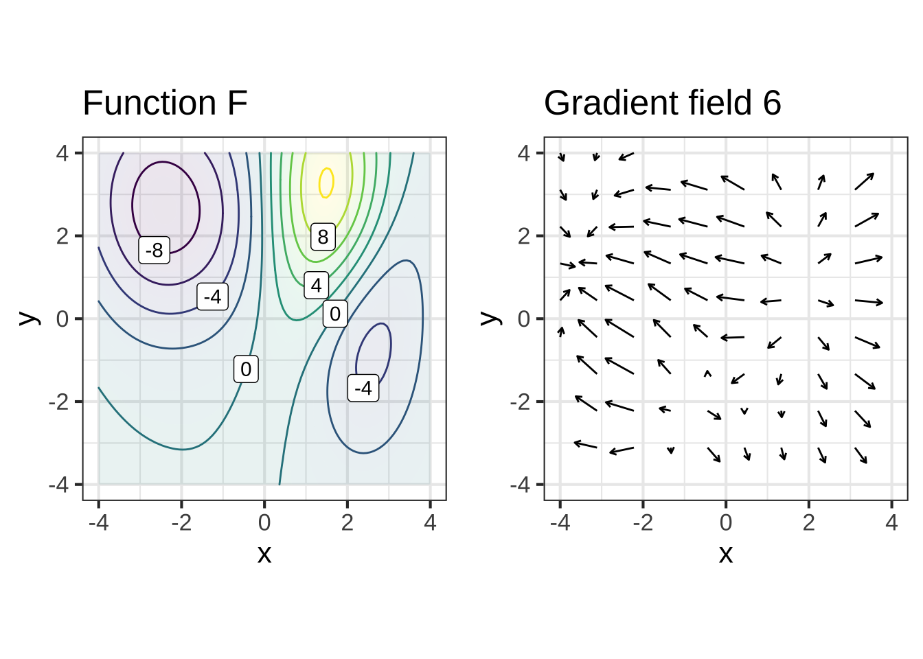
Each of the figures below shows a contour plot and a gradient field. For some of the figures, the contour plot and the gradient field show the same function, for others they do not. Your task is to identify whether the contour plot and the gradient field are of the same or different functions.

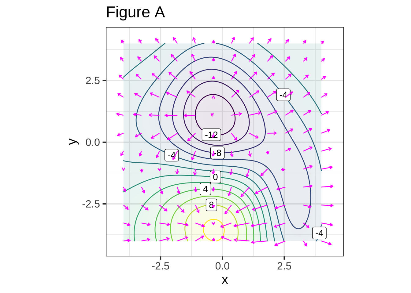
For Figure A, do the contour plot and the gradient field show the same function? 



(x )  Yes
( )  No

[[Right!]]

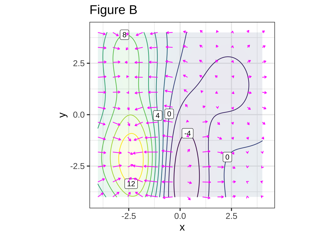
For Figure B, do the contour plot and the gradient field show the same function? 



(x )  Yes
( )  No

[[Good.]]

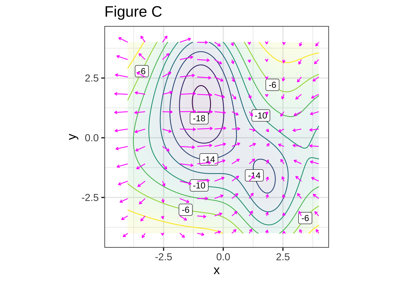
For Figure C, do the contour plot and the gradient field show the same function? 



( )  Yes
(x )  No

[[Good.]]

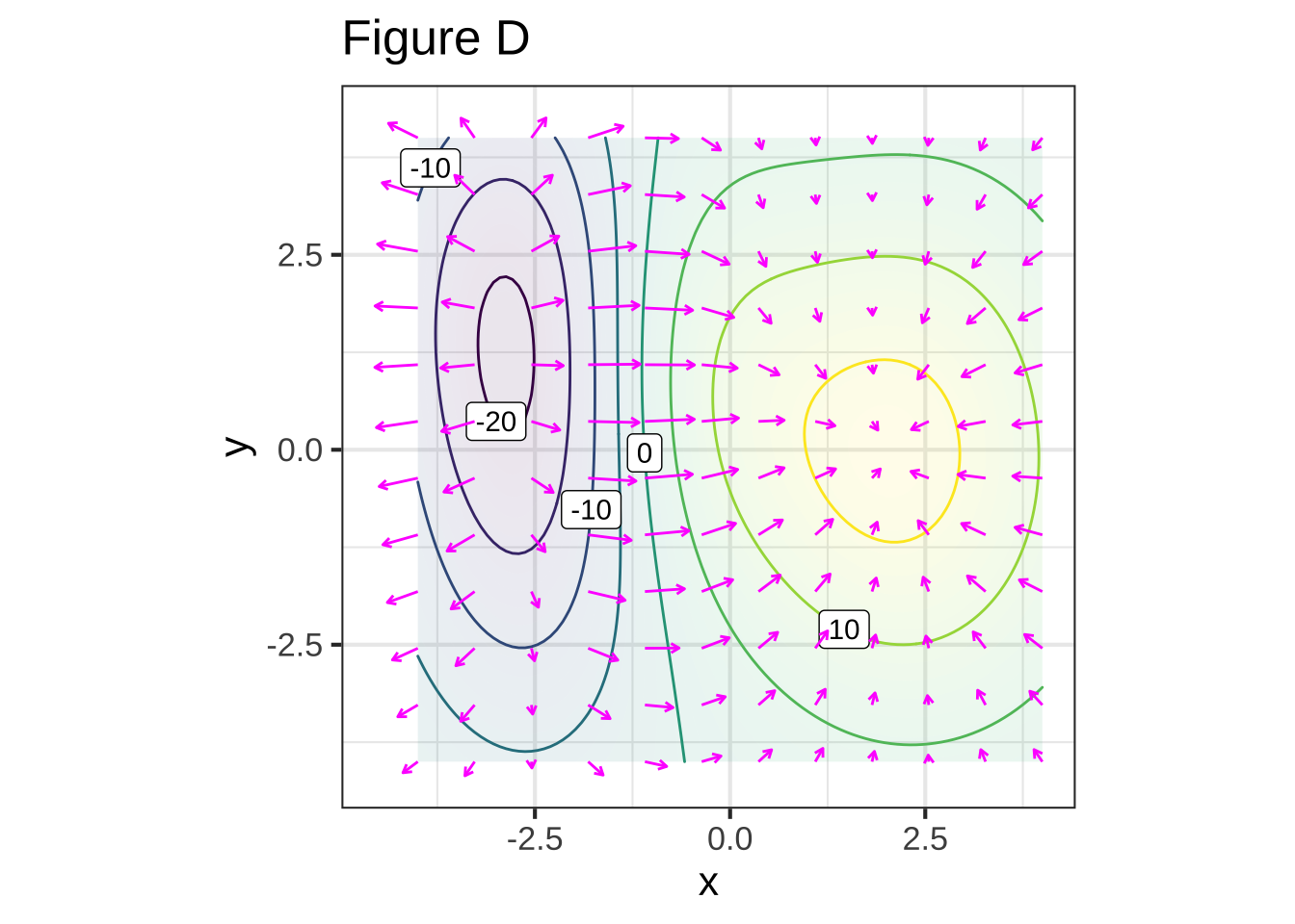
For Figure D, do the contour plot and the gradient field show the same function? 



(x )  Yes
( )  No

[[Right!]]

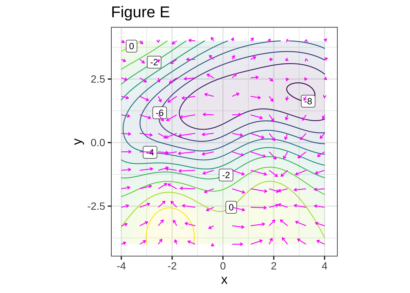
For Figure E, do the contour plot and the gradient field show the same function? 



( )  Yes
(x )  No

[[Excellent!]]

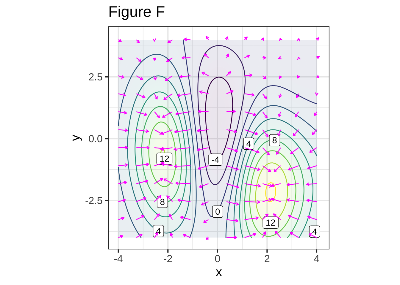
For Figure F, do the contour plot and the gradient field show the same function? 



(x )  Yes
( )  No

[[Excellent!]]

Exercise 24.08: lkwciw

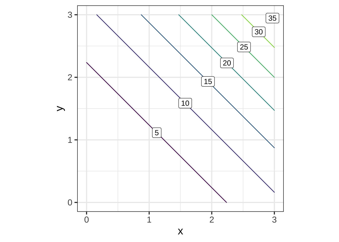
Here is a contour plot of a function \(g(x,y)\). You will be presented with several gradient fields. Your task is to determine whether the gradient field corresponds to the contour plot and, if not, say why not.

## Warning: Removed 19 rows containing missing values (geom_segment).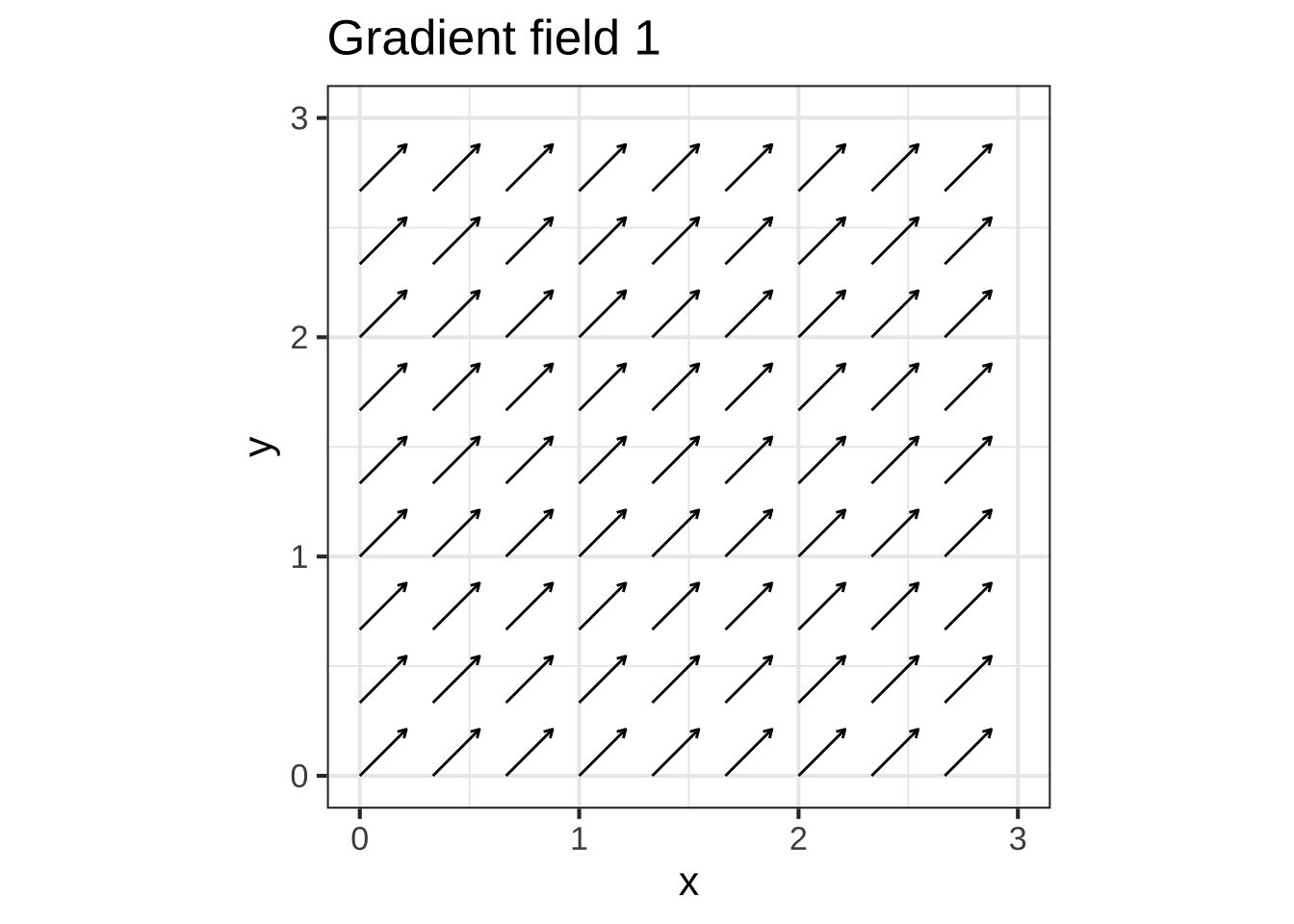

What's wrong with gradient field 1? 



( )  arrows point down the hill instead of up it
(x )  magnitude of arrows are wrong, but direction is right
( )  arrows don't point in the right direction
( )  nothing is wrong

[[Right!]]

## Warning: Removed 18 rows containing missing values (geom_segment).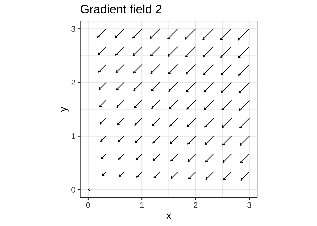

What's wrong with gradient field 2? 



(x )  arrows point down the hill instead of up it
( )  magnitude of arrows are wrong, but direction is right
( )  arrows don't point in the right direction
( )  nothing is wrong

[[Excellent!]]

## Warning: Removed 19 rows containing missing values (geom_segment).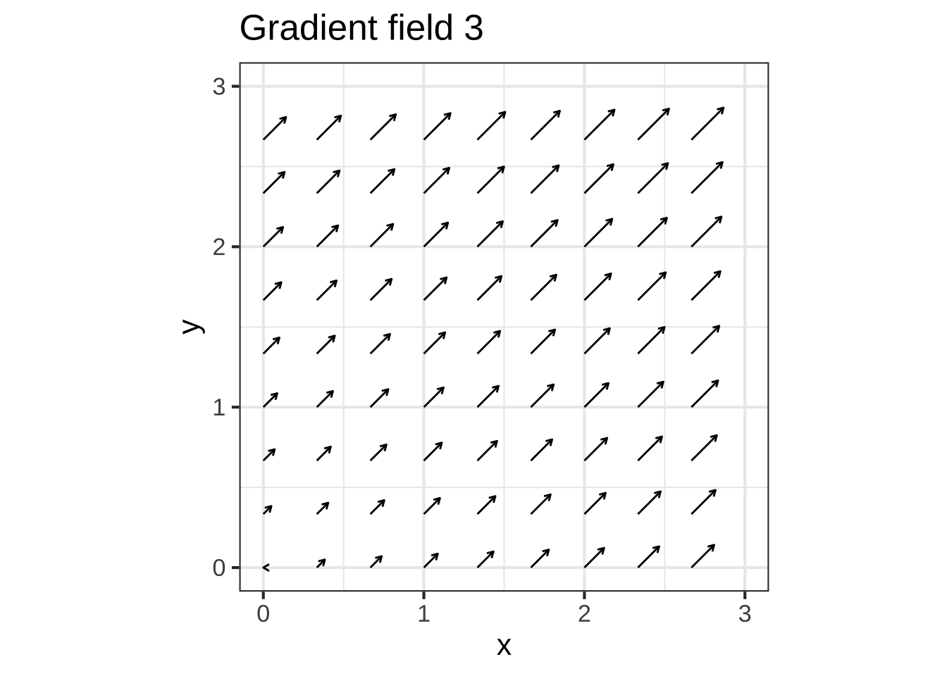

What's wrong with gradient field 3? 



( )  arrows point down the hill instead of up it
( )  magnitude of arrows are wrong, but direction is right
( )  arrows don't point in the right direction
(x )  nothing is wrong

[[Correct.]]

## Warning: Removed 19 rows containing missing values (geom_segment).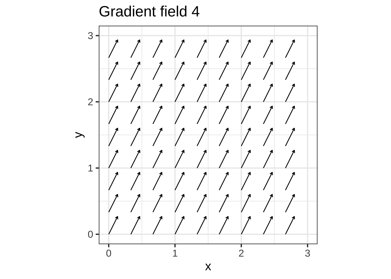

What's wrong with gradient field 4? 



( )  arrows point down the hill instead of up it
( )  magnitude of arrows are wrong, but direction is right
(x )  arrows don't point in the right direction
( )  nothing is wrong

[[Good.]]

Exercise 24.10: wkd83

Here are contour maps and gradient fields of several functions with input \(x\) and \(y\). But any row of graphs may show two different functions. Your job is to match the contour plot with the gradient field, which may be in another row.

Which contour plot matches gradient field 1? 



( )  A
( )  B
( )  C
( )  D
( )  E
(x )  F

[[Excellent!]]

Which contour plot matches gradient field 2? 



(x )  A
( )  B
( )  C
( )  D
( )  E
( )  F

[[Correct.]]

Which contour plot matches gradient field 3? 



( )  A
( )  B
( )  C
(x )  D
( )  E
( )  F

[[Good.]]

Which contour plot matches gradient field 4? 



( )  A
( )  B
(x )  C
( )  D
( )  E
( )  F

[[Good.]]

Which contour plot matches gradient field 5? 



( )  A
( )  B
( )  C
( )  D
(x )  E
( )  F

[[Nice!]]

Which contour plot matches gradient field 6? 



( )  A
(x )  B
( )  C
( )  D
( )  E
( )  F

[[Good.]]

Exercise 24.12: tPsfoR

Using the gradient field depicted below, figure out the sign of the partial derivatives at the labeled points. We’ll use “neg” to refer to negative partial derivatives, “pos” to refer to positive partial derivatives, and “zero” to refer to partials that are so small that you can’t visually distinguish them from zero.

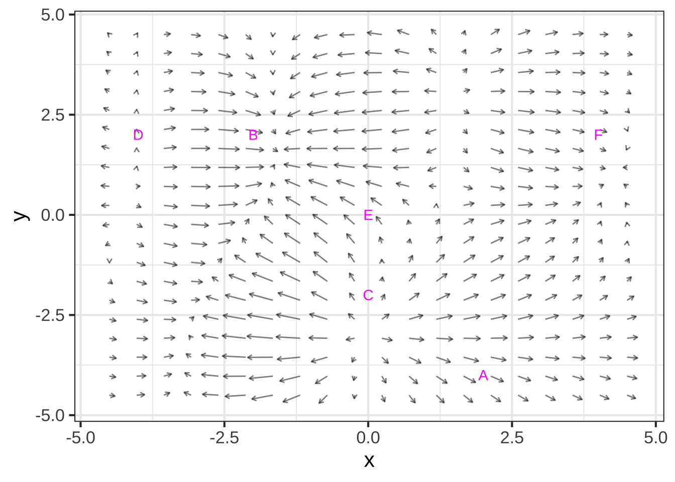
Which is $$\partial_y f$$ at point A? 



(x )  neg
( )  zero
( )  pos

[[Excellent!]]

Which is $$\partial_x f$$ at point A? 



( )  neg
( )  zero
(x )  pos

[[Nice!]]

Which is $$\partial_x f$$ at point B? 



( )  neg
( )  zero
(x )  pos

[[Nice!]]

Which is $$\partial_x f$$ at point C? 



( )  neg
(x )  zero
( )  pos

[[Nice!]]

Which is $$\partial_y f$$ at point E? 



( )  neg
( )  zero
(x )  pos

[[Good.]]

Which is $$\partial_x f$$ at point E? 



(x )  neg
( )  zero
( )  pos

[[Excellent!]]

At which letter are both the partial with respect to $$x$$ and the partial with respect to $$y$$ negative.? 



( )  A
( )  B
( )  C
( )  D
( )  E
( )  F
(x )  none of them

[[Nice!]]

Exercise 24.14: vkdlw

For almost everyone, a house is too expensive to buy with cash, so people need to borrow money. The usual form of the loan is called a “mortgage.” Mortgages extend over many years and involve paying a fixed amount each month. That amount is calculated so that, by paying it each month for the duration of the mortgage, the last payment will completely repay the amount borrowed plus the accumulated interest.

The monthly mortgage payment in dollars, \(P\), for a house is a function of three variables, \[P(A, r, N)\] where \(A\) is the amount borrowed in dollars, \(r\) is the interest rate (percentage points per year), and \(N\) is the number of years before the mortgage is paid off.

A studio apartment is selling for $220,000. You will need to borrow $184,000 to make the purchase.

Suppose $$P(184000,4,10) = 2180.16$$.  What does this tell you in financial terms? 



(x )  The monthly cost of borrowing $$184,000 for 10 years at 4% interest per year.
( )  The monthly cost of borrowing $$184,000 for 4 years at 10% interest per year.
( )  The annual cost of the mortgage at 4% interest for 10 years.
( )  The annual cost of the mortgage at 10% interest for 4 years

[[Correct.]]

The next two questions involve what happens to the monthly mortgage payments if you change either the amount or duration of the mortgage. (Hint: Common sense works wonders!)

What would you expect about the quantity $$\partial P / \partial A$$, the partial derivative of the monthly mortgage payment with respect to the amount of money borrowed? 



(x )  It's positive
( )  It's zero
( )  It's negative

[[If you borrow more money, holding mortgage duration and interest rate constant, you are going to have to pay more each month.]]

What would you expect about the quantity $$\partial P / \partial N$$, the partial derivative of the monthly mortgage payment with respect to the number of years the mortgage lasts? 



( )  It's positive
( )  It's zero
(x )  It's negative

[[If you borrow the same amount of money at the same interest rate, but have more years to pay it back, your monthly payment will be smaller.]]

Suppose $$\partial_r P (184000,4,30) =$$ $$145.65.  What is the financial significance of the number $$145.65?? 



( )  If the interest rate $$r$$ went up from 4 to 5, the monthly payment would increase by $$145.65.
( )  If the interest rate $$r$$ went up from 4 to 4.001, the monthly payment would increase by $$145.65.
(x )  If the interest rate $$r$$ went up from 4 to 4.001, the monthly payment would increase by $$0.001     imes $$145.65.

[[You might think that nobody would be concerned about such a small increase in interest rate. But knowing the result for each very small increase allows us to calculate what would be the impact of a large increase by a process  called *integration*.]]

Exercise 24.16: 72ldw

In economic theory, the quantity of the demand for any good is a decreasing function of the price of that good and an increasing function of the price of a competing good.

The classical example is that apple juice competes with orange juice. The demand for orange juice is in units of thousands of liters of orange juice. The price is in units of dollars per liter.

Here’s a graph with the input variables unlabeled. The contour labels indicate the demand for orange juice.

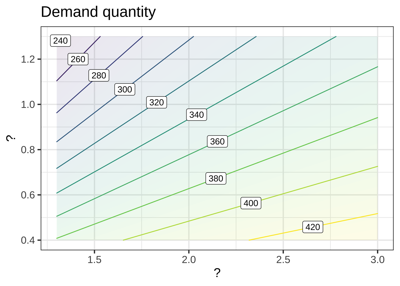
The concept of partial derivatives makes it much easier to think about the situation. There are two partial derivative functions relevant to the function in the graph. Well denote the input variables apple and orange, but remember that these are the prices of those commodities in dollars per liter.

• \(\partial_\text{apple} \text{demand}()\) – how the demand changes when apple-juice price goes up, holding orange-juice price constant. (Another notation that is more verbose but perhaps easier to read \(\frac{\partial\, \text{demand}}{\partial\,\text{apple}}\))
• \(\partial_\text{orange} \text{demand}()\) – how the demand changes when orange-juice price goes up, holding apple-juice price constant. (Another notation: \(\frac{\partial\, \text{demand}}{\partial\,\text{orange}}\))

Notice that the notation names both the output and the single input which is to be changed–the other inputs will be held constant.

The first paragraph of this problem gives the economic theory which amounts to saying that one of the partial derivatives is positive and the other negative.

What is the proper translation of the notation $$\partial_\text{apple}\text{demand}()$$? 



(x )  The partial derivative of orange-juice  demand *with repect to* apple-juice price
( )  The partial derivative of apple-juice price *with respect to* demand for orange juice
( )  The partial derivative of apple-juice demand *with respect to* price of apple juice
( )  The partial derivative of orange-juice price *with respect to* apple-juice price.

[[Correct.]]

According to the economic theory described above, one of the partial derivatives will be positive and the other negative. Which will be *positive*. 



(x )  $$\partial_\text{apple}  \text{demand}()$$
( )  $$\partial_\text{orange} \text{demand}()$$

[[Right!]]

What does the vertical axis measure? 



(x )  Price of orange juice
( )  Quantity of apple juice
( )  Quantity of orange juice
( )  Price of apple juice

[[Nice!]]

Consider the magnitude (absolute value) of the partial derivative of demand with respect to orange-juice price. Is this magnitude greater toward the top of the graph or the bottom? 



(x )  top
( )  bottom
( )  neither

[[Right!]]

Exercise 24.18: oekse

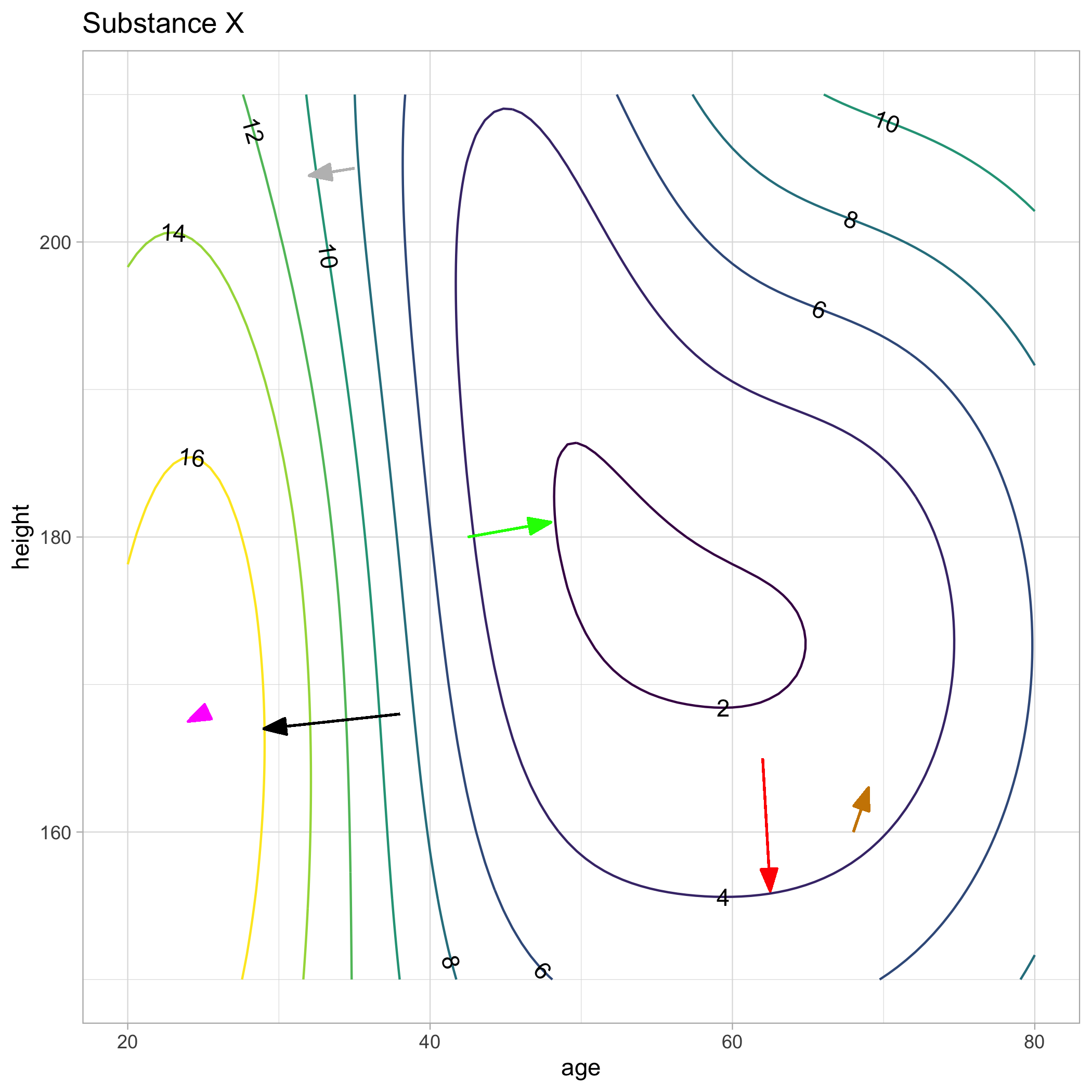
The contour plot of function \(g(y, z)\) is overlaid with vectors. The black vector is a correct representation of the gradient (at the root of the vector). The other vectors are also supposed to represent the gradient, but might have something wrong with them (or might not). You’re job is to say what’s wrong with each of those vectors.

What's wrong with the **red** vector? 



( )  nothing
(x )  too long
( )  too short
( )  points downhill
( )  points uphill
( )  wrong direction entirely

[[The red vector is located in a place where the function is almost level. You can tell this because the contour lines are spaced far apart. The magnitude of the gradient will be small in such an area. But here, the red vector is even longer than the black vector, even though black is in a very steep area (with closely spaced contours).]]

What's wrong with the **green** vector? 



( )  nothing
( )  too long
( )  too short
(x )  points downhill
( )  points uphill
( )  wrong direction entirely

[[The root of the green vector is near contour=4, the head at contour=2. So the vector is incorrectly pointing downhill. Gradients point in the steepest direction uphill.]]

What's wrong with the **blue** vector? 



(x )  nothing
( )  too long
( )  too short
( )  points downhill
( )  points uphill
( )  wrong direction entirely

[[Nice!]]

What's wrong with the **orange** vector? 



( )  nothing
( )  too long
( )  too short
( )  points downhill
( )  points uphill
(x )  wrong direction entirely

[[Gradient vectors should be perpendicular to nearby contours and should point uphill. The orange vector is neither]]

What's wrong with the **gray** vector? 



( )  nothing
( )  too long
(x )  too short
( )  points downhill
( )  points uphill

[[The function is practically as steep at the root of the gray vector as it is at the root of the black vector. (You can tell this from the spacing of the contour lines.) So the magnitude of the gray vector should be just about the same as the magnitude of the black vector.]]

Exercise 24.20: ZQlUv4

Let’s return to the water skier in Section 24.5. When we left her, the rope was being pulled in at 10 feet per second and her corresponding speed on the water was 10.05 feet per second. The relationship between the rope speed and the skier’s speed was \[dx = \frac{L}{x} dL\] and, due to the right-angle configuration of the tow system, \(x^2 = L^2 - H^2\).

What happens to \(dx\) as \(L\) gets smaller with \(dL\) being the same? We need to keep in mind that \(dx\) depends on three things: \(dL\), \(L\), and \(x\). But we can substitute in the Pythagorean relationship between \(x\), \(L\), and (fixed) \(H\) to get \[dx = \frac{L}{\strut\sqrt{L^2 - H^2}}\ dL\ .\] This is bad news for the skier who holds on too long! As \(L\) approaches \(H\), the rope becomes more and more vertical and the skier’s water speed becomes greater and greater, approaching \(\infty\) as \(L \rightarrow H\).

You, an engineer brought in to solve this dangerous possibility, have proposed to have the winch slow down as the rope is reeled in. How should the speed of the rope be set so that the skier’s water speed remains safely constant?

What formula for $$dL$$ will allow $$dx$$ to stay constant at a value $$v$$? 



( )  $$dL = dx$$
(x )  $$dL = v \sqrt{L^2 - H^2}{L}$$
( )  $$dL = v \sqrt{L^2 - H^2}$$
( )  There is no such formula.

[[The roop speed will get slower and slower, coming to zero when $$L = H$$]]