31 Symbolic anti-differentiation
You have already learned how to write down, by sight, the anti-derivative of the many of the pattern-book functions. As a reminder, here is an (almost) complete list of the derivatives and anti-derivatives of the pattern-book functions.
| \(\partial_x f(x)\) | \(f(x)\) | \(\int f(x) dx\) |
|---|---|---|
| \(e^x\) | \(e^x\) | \(e^x\) |
| \(\sin(x+\pi/2)\) | \(sin(x)\) | \(\sin(x - \pi/2)\) |
| \(p x^{p-1}\) | power-law \(x^p\) | \(\frac{1}{p+1} x^{p+1}\) |
| \(\ \ \ \ 2x\) | \(\ \ \ \ x^2\) | \(\frac{1}{3} x^3\) |
| \(\ \ \ \ 1\) | \(\ \ \ \ x\) | \(\frac{1}{2} x^2\) |
| \(\ \ \ \ 0\) | \(\ \ \ \ 1\) | \(x\) |
| \(\ \ \ \ -x^{-2}\) | \(\ \ \ \ 1/x\) | \(\ln(x)\) |
| \(1/x\) | \(\ln(x)\) | \(x \left(\strut\ln(x) - 1\right)\) |
| \(-x \dnorm(x)\) | \(\dnorm(x)\) | \(\pnorm()\) |
| \(\dnorm(x)\) | \(\pnorm(x)\) | See below. |
You can see that the derivatives and anti-derivatives of the pattern-book functions can be written in terms of the pattern-book functions. The left column contains the symbolic derivatives of the pattern book functions. The right column contains the symbolic anti-derivatives. We call them “symbolic,” because they are written down with the same kind of symbols that we use for writing the pattern-book functions themselves.49
We’re stretching things a bit by including \(\dnorm(x)\) and \(\pnorm(x)\) among the functions that can be integrated symbolically. As you’ll see later, \(\dnorm(x)\) is special when it comes to integration.
Think of the above table as the “basic facts” of differentiation and anti-differentiation. It’s well worth memorizing the table since it shows many of the relationships among the functions that are central to this book. You may prefer to use the name \(\cos(x)\) to refer to \(\sin(x + \pi/2)\) and to use \(-\cos(x)\) instead of \(\sin(x - \pi/2)\).
For differentiation, any function that can be written using combinations of the pattern-book functions by multiplication, composition, and linear combination has a derivative that can be written using the pattern-book functions. So a complete story of symbolic differentiation is told by the above table and the differentiation rules:
linear combination: \(\partial_x \left[{\strut}a\, f(x) + b\, g(x)\right] = a\, \partial_x f(x) + b\, \partial_x g(x)\)
product: \(\partial_x \left[{\strut}f(x)\cdot g(x)\right] = g(x) \partial_x f(x) + f(x) \partial_x g(x)\)
composition: \(\partial_x \left[{\strut}f(g(x))\right] = \left[\partial_y f(g(x))] \cdot \partial_x g(x)\)
This chapter is about the analogous rules for anti-differentiation. The anti-differentiation rule for linear combination is simple: essentially the same as the rule for differentiation.
\[\int \left[\strut a\, f(x) + b\, g(x)\right] = a\!\int\! f(x) dx + b\!\int\! g(x) dx\] How about the rules for function products and for composition? The surprising answer is that there are no such rules. There is no template analogous to the product and chain rules for derivatives, that can consistently be used for anti-derivatives. What we have instead are techniques of integration, somewhat vague rules that will sometimes guide a successful search for the anti-derivative, but often will lead you astray.
Indeed, there are many functions for which a symbolic anti-derivative cannot be constructed from compositions and/or multiplication of pattern-book functions that can be written using pattern-book functions.50
Fortunately, we already know the symbolic anti-derivative form of many functions. We’ll call those the cataloged functions, but this is not a term in general use in mathematics. For functions not in the catalog, it is non-trivial to find out whether the function has a symbolic anti-derivative or not. This is one reason why the techniques of integration do not always provide a result.
The following sections provide an overview of techniques of integration. We start with a description of the cataloged functions and direct you to computer-based systems for looking up the catalog. (These are almost always faster and more reliable than trying to do things by hand.) Then we introduce a new interpretation of the notation for anti-differentiation: differentials. This interpretation makes it somewhat easier to understand the major techniques of integration: substitution and integration by parts. We’ll finish by returning to a setting where symbolic integration is easy: polynomials.
Remember that, even if we cannot always find a symbolic anti-derivative, that we can always construct a numerical anti-derivative that will be precise enough for almost any genuine purpose.
31.1 The cataloged functions
In a traditional science or mathematics education, students encounter (almost exclusively) basic functions from a mid-sized catalog. For instance: \(\sqrt{\strut\_\_\_\ }\), \(\sin()\), \(\cos()\), \(\tan()\), square(), cube(), recip(), \(\ln()\), \(\exp()\), negate(), gaussian(), and so on. This catalog also includes some functions that take two arguments but are traditionally written without using parentheses. For instance, \(a+b\) doesn’t look like a function but is entirely equivalent to \(+(a, b)\). Others in this class are \(\times(\ ,\ )\), \(\div(\ , \ )\), \(-(\ ,\ )\), and ^( , ).
The professional applied mathematician’s catalog is much larger. You can see an example published by the US National Institute of Standards and Technology as the Digital Library of Mathematical Functions. (Almost all of the 36 chapters in this catalog, important though they be, are highly specialized and not of general interest across fields.)
There is a considerable body of theory for these cataloged functions, which often takes the form of relating them to one another. For instance, \(\ln(a \times b) = \ln(a) + \ln(b)\) demonstrates a relationship among \(\ln()\), \(+\) and \(\times\). Along the same lines of relating the cataloged functions to one another is \(\partial_x \sin(x) = \cos(x)\) and other statements about derivatives such as those listed in Section 19.4.6.
Simply to illustrate what a function catalog looks like, Figure 31.1 shows a page from an 1899 handbook entitled A Short Table of Integrals.
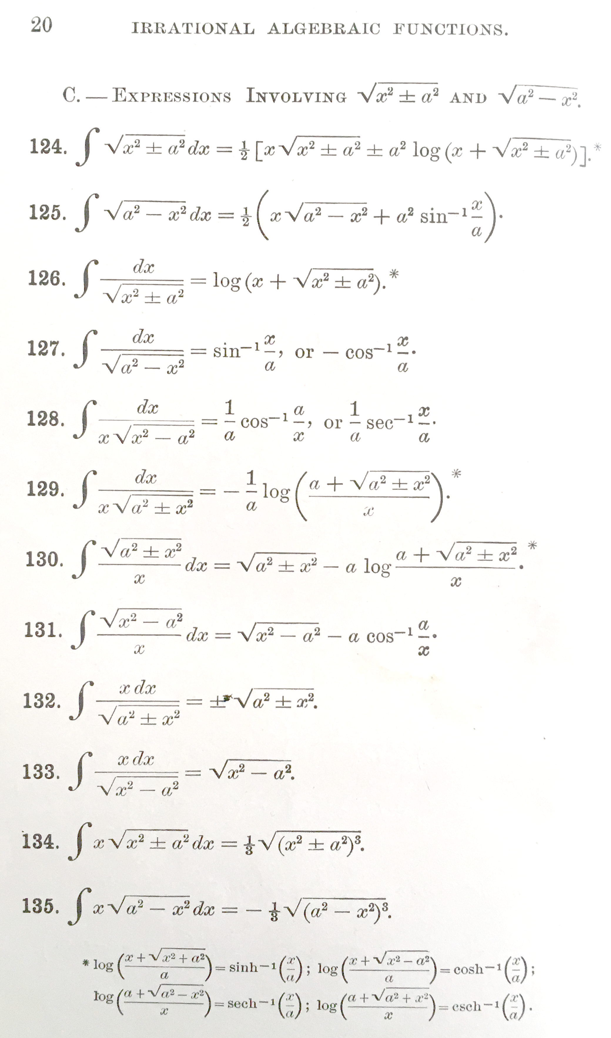
Figure 31.1: Entries 124-135 from A Short Table of Integrals (1899) by Benjamin Osgood Pierce. The book includes 938 such entries.
The use of cataloged functions is particularly prevalent in textbooks, so the quantitatively sophisticated student will encounter symbolic anti-derivatives of these functions throughout his or her studies.
The cataloged functions were assembled with great effort by mathematicians over the decades. The techniques and tricks they used to find symbolic anti-derivatives are not part of the everyday experience of technical workers, although many mathematically minded people find them a good source of recreation.
Calculus textbooks that include extensive coverage of the techniques and tricks should be understood as telling a story of the historical construction of catalogs, rather than conveying skills that are widely used today. In a practical sense, when the techniques are needed, it’s more reliable to access them via computer interface such as WolframAlpha, as depicted in Figure 31.2.
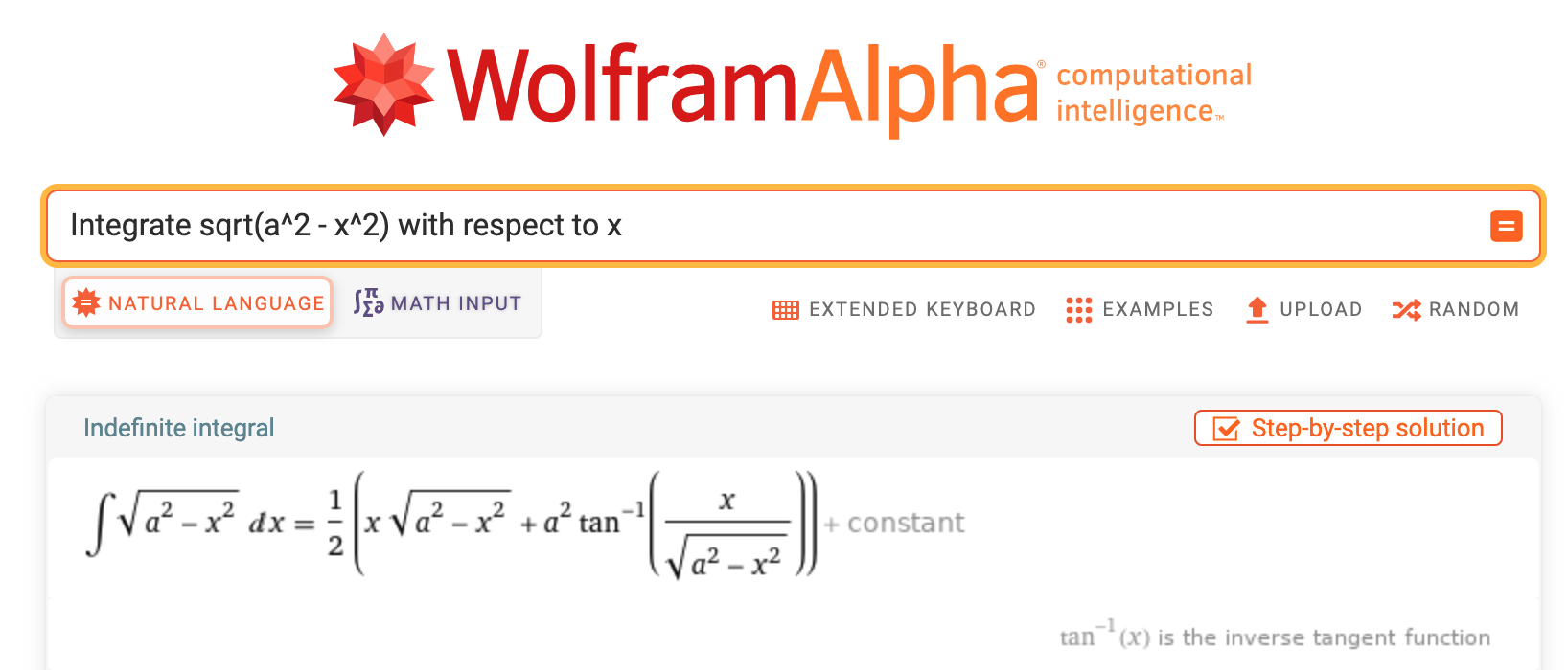
Figure 31.2: Pierce’s entry 125 as computed by the WolframAlpha system.
The systems can do a good job identifying cases where the techniques will not work. In such systems, they provide the anti-derivative as constructed by numerical integration. The R/mosaic antiD() function works in this same way, although its catalog contains only a tiny fraction of the functions found in professional systems. (But then, only a tiny fraction of the professional cataloged function are widely used in applied work.)
31.2 Differentials
Breathing some life into the symbol \(dx\) will help in understanding the algebra of techniques for anti-differentiating function compositions and products. We’ve thus far presented \(dx\) as a bit of notation: punctuation for identifying the with-respect-to input in anti-derivatives. That is, in interpreting a sequence of symbols like \(\int f(x,t) dx\), we’ve parsed the sequence of symbols into three parts:
\[\underbrace{\int}_{\text{integral sign}} \overbrace{f(x, t)}^{\text{function to be anti-differentiated}} \underbrace{dx}_{\text{'with respect to'}}\]
By analogy, the English sentence
\[\text{We loaded up on snacks.}\]
consists of five parts: the five words in the sentence.
But you can also see “We loaded up on snacks” as having three parts:
\[\underbrace{\text{We}}_{\text{subject}}\ \overbrace{\text{loaded up on}}^{\text{verb}}\ \ \ \underbrace{\text{snacks}}_{\text{object}}\]
Likewise, the integrate sentence can be seen as consisting of just two parts:
\[\underbrace{\int}_{\text{integral sign}} \overbrace{f(x, t) dx}^{\text{differential}}\]
A differential corresponds to the little sloped segments that we add up when calculating a definite integral numerically using the slope function visualization. That is \[\underbrace{\int}_{\text{Sum}} \underbrace{\overbrace{f(x,t)}^\text{slope of segment}\ \ \overbrace{dx}^\text{run}}_\text{rise}\]
A differential is a genuine mathematical object and is used, for example, in analyzing the geometry of curved spaces, as in the Theory of General Relativity. But this is well beyond the scope of this introductory calculus course.  3710
3710
Our use here for differentials will be to express rules for anti-differentiation of function compositions and products.
You should be thinking in terms of differentials when you see a sentence like the following:
“In \(\int \sin(x) \cos(x) dx\), make the substitution \(u = \sin(x)\), implying that \(du = \cos(x) dx\) and getting \(\int u du\), which is simple to integrate.”
The table gives some examples of functions and their differentials. “w.r.t” means “with respect to.”
| Function | derivative | w.r.t. | differential |
|---|---|---|---|
| \(v(x) \equiv x\) | \(\partial_x v(x) = 1\) | x | \(dv = dx\) |
| \(u(x) \equiv x^2\) | \(\partial_x u(x) = 2x\) | x | \(du = 2x dx\) |
| \(f(x) \equiv \sin(x)\) | \(\partial_x f(x) = \cos(x)\) | x | \(df = \cos(x)dx\) |
| \(u(x) \equiv e^{3 x}\) | \(\partial_x u(x) = 3 e^{3 x}\) | x | \(du = 3 e^{3 x} dx\) |
| \(g(x) \equiv t^3\) | \(\partial_t v(t) = 3 t^2\) | t | \(dg = 3 t^2 dt\) |
As you can see, the differential of a function is simply the derivative of that function followed by the little \(dx\) or \(dt\) or whatever is appropriate for the “with respect to” variable.
Notice that the differential of a function is not written with parentheses: The function \(u(x)\) corresponds to the differential \(du\).
Example 31.1 What is the differential of \(\sin(x)\)?
As we’ve seen, \(\partial_x \sin(x) = cos(x)\). For form the differential of \(\sin()\), take the derivative and suffix it with a \(dx\) (since \(x\) is the name of the input):
\[\cos(x)\ dx\]
31.3 U-substitution
There is little reason to use \(\partial_t\) and \(\int \left[\right]dt\) to cancel each other out, but it is the basis of an often successful strategy—u-substitution—for finding anti-derivatives symbolically. Here’s the differentiate/integrate algorithm behind u-substitution. 3725
- Pick a function \(f()\) and another function \(g()\). Typically \(f()\) and \(g()\) belong to the family of basic modeling functions, e.g. \(e^x\), \(\sin(t)\), \(x^n\), \(\ln(x)\), and so on. For the purpose of illustration, we’ll use \(f(x) = \ln(x)\) and \(g(t) = \cos(t)\).
- Compose \(f()\) with \(g()\) to produce a new function \(f(g())\) which, in our case, will be \(\ln(\cos(t))\).
- Use the chain rule to find \(\partial_t f(g(t))\). In the example, the derivative of \(\ln(x)\) is \(1/x\), the derivative of \(g(t)\) is \(-\sin(t)\). By the chain rule, \[\partial_t f(g(t)) = - \frac{1}{g(t)} \sin(t)= - \frac{\sin(t)}{\cos(t)} = - \tan(t)\] 3730
In a sense, we have just watched a function give birth to another through the straightforward process of differentiation. Having witnessed the birth, we know who is the integration parent of \(\tan(t)\), namely \(\int \tan(t) dt = \ln(\cos(t)\). For future reference, we might write this down in our diary of integrals:
\[\int \tan(t) dt = - \ln(\cos(t)) + C\]
Saving this fact in your diary is helpful. The next time you need to find \(\int \tan(x) dx\), you can look up the answer (\(-\ln(\cos(x)) + C\)) from your diary. If you use \(\int \tan(x) dx\) a lot, you will probably come to memorize the answer, just as you have already memorized that \(\int \cos(t) dt = \sin(t)\) (a fact that you actually will use a lot in the rest of this course). 3735
Now for the u-substitution game. The trick is to take a problem of the form \(\int h(t) dt\) and extract from \(h(t)\) two functions, an \(f()\) and a \(g()\). You’re going to do this so that \(h(t) = \partial_t F(g(t))\), where \(\partial_x F(x) = f(x)\) Once you’ve done this, you have an answer to the original integration question: \(\int h(t) dt = F(g(t)) + C\). 3740
::: {.example data-latex=""}
Task: Evaluate the definite integral \(\int \frac{\sin(\ln(x))}{x} dx\).
You don’t know ahead of time that this is an integral amenable to solution by u-substitution. For all you know, it’s not. So before you start, look at the function to see if it one of those for which you already know the anti-derivative, for example any of the pattern-book functions or their parameterized cousins the basic modeling functions. 3745
If so, you’ve already memorized the answer and you are done. If not …
Assume for a moment—without any guarantee that this will work, mind you—that the answer can be built using u-substitution. You will therefore look hard at \(h()\) and try to see in it a plausible form that looks like the derivative of some \(f(g(x))\). 3750
In the problem at hand, we can readily see something of the form \(f(g(x))\) in the \(\sin(\ln(x))\). This immediately gives you a candidate for \(g(x)\), namely \(g(x)\equiv \ln(x)\) We don’t know \(f()\) yet, but if \(g()\) is the right guess, and if u-substitution is going to work, we know that \(f()\) has to be something that produces \(\sin()\) when you differentiate it. That’s \(-\cos()\). So now we have a guess \[h_\text{guess}(x) = -\cos(\ln(x)) \partial_x \ln(x) = - \cos(\ln(x)) \frac{dx}{x}\] 3755
If this guess matches the actual \(h()\) then you win. The answer to \(\int h(x) dx\) will be \(f(g(x)) = -\cos(\ln(x))\). If not, see if there is any other plausible guess for \(g(x)\) to try. If you can’t find one that works, try integration by parts.
31.4 Integration by parts
Integration by parts applies to integrals that are recognizably of the form \[\int f(x) g(x) dx\] Step 1: Split up the integrand into an \(f(x)\) and a \(g(x)\) multiplied together. That is, split the integrand into parts that are multiplied together. The way we wrote the integrand, this was trivial.
Step 2: Pick one of \(f(x)\) or \(g(x)\). Typically, you pick the one that has a dead-easy anti-derivative. For our general description, let’s suppose this is \(g(x)\) which has anti-derivative \(G(x)\) (where we know \(G()\)).
Step 3: Construct a helper function \(h(x) \equiv f(x) G(x)\). This requires no work, since we’ve already identified \(f(x)\) and \(G(x)\) in step (2).
Step 4: Find \(\partial_x h(x)\). It’s always easy to find derivatives, and here we just use the product rule: \[\partial_x h(x) = \partial_x f(x) \cdot G(x) + f(x)\cdot\partial_x G(x)\] We know from the way we constructed \(G(x)\) that \(\partial_x G(x) = g(x)\), so the equation is \[\partial_x h(x) = \partial_x f(x) \cdot G(x) + f(x)\cdot g(x)\]
Step 5: Anti-differentiate both sides of the previous equation. From the fundamental theorem of calculus, we know how to do the left side of the equation. \[\int \partial_x h(x) = h(x) \equiv f(x)g(x)\] The right side of the equation has two parts: \[\int \left[{\large\strut}\partial_x f(x) \cdot G(x) + f(x)\cdot g(x)\right]dx = \underbrace{\int \partial_x f(x) \cdot G(x) dx}_\text{Some NEW integral!}\ \ \ \ + \underbrace{\int f(x) g(x) dx}_\text{The original integral we sought!}\] Putting together the left and right sides of the equation, and re-arranging gives us a new expression for the original integral we sought to calculate: \[\text{Integration by parts re-arrangement}\\\underbrace{\int f(x) g(x) dx}_\text{The original integral we sought.} = \underbrace{f(x) g(x)}_\text{We know this!} - \underbrace{\int \partial_x f(x) \cdot G(x) dx}_\text{Some NEW integral!}\] It may seem that we haven’t accomplished much with this re-organization. But we have done something. We took a problem we didn’t otherwise know how to solve (that is \(\int f(x) g(x) dx\)) and broke it down into two parts. One is very simple. The other is an integral. If we’re clever in picking \(g()\) and lucky, we’ll be able to figure out the new integral and, thereby, we’ll have computed the original integral. But everything depends on cleverness and luck!
Example 31.2 Task: Find \(\int x \cos(x) dx\).
An obvious choice for the two parts is \(x\) and \(\cos(x)\). But which one to call \(g(x)\). We’ll just guess and say \(g(x)\equiv \cos(x)\) which implies \(G(x) = \sin(x)\). The helper function is \(h(x) \equiv f(x) G(x) = x \sin(x)\).
Differentiating \(h(x)\) can be done by the product rule. \[\partial_x h(x) = \sin(x) + x \cos(x)\ .\] Now anti-differentiate both sides of the above, the left side by the fundamental theorem of algebra and the right side by other means: \[\int \partial_x h(x) = h(x) = x \sin(x)= \underbrace{\int\sin(x)dx}_{-\cos(x)} + \underbrace{\int x \cos(x) dx}_\text{The original integral}\] Re-arranging gives the answer \[\underbrace{\int x \cos(x) dx}_\text{The original integral} = x \sin(x) + \cos(x) + C\] The constant of integration \(C\) needs to be included to make the equality true.
To confirm the result, you can differentiate the right-hand side; differentiation is always easy.
Alternatively, we can check numerically if \(\int x \cos(x) dx - (x\sin(x)+cos(x))\) is really a constant.
F1 <- antiD(x*cos(x) ~ x)
F2 <- makeFun(x*sin(x) + cos(x) ~ x)
slice_plot(F1(x) - F2(x) ~ x, domain(x=c(-5,5)))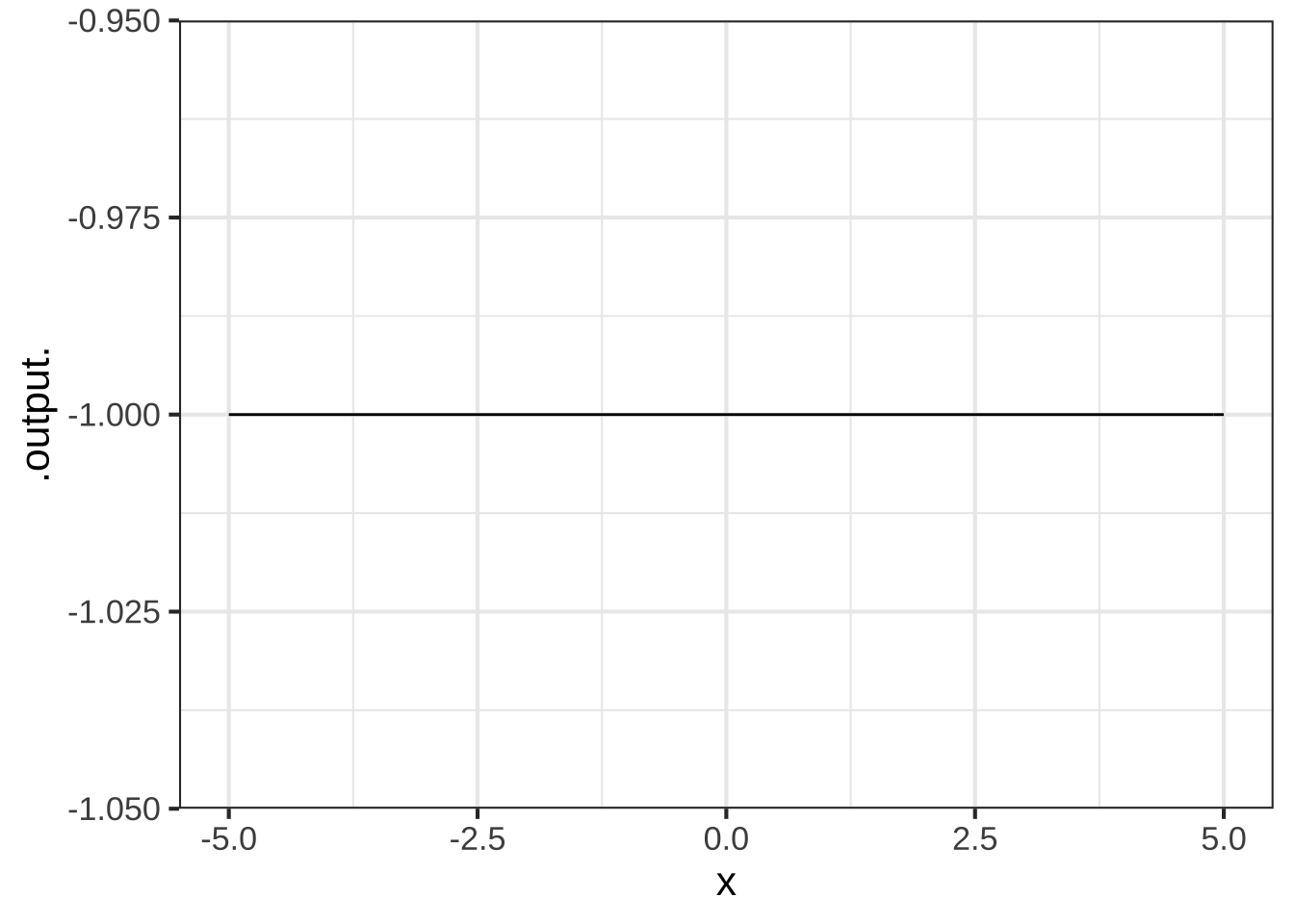 Yes! The graph shows a constant function: \(C\).
Example 31.3 Task: Find \(\int \ln(x) dx\).
The easy solution is to recognize that the anti-derivative of \(\ln(x)\) is contained in the table at the top of the chapter. But let’s try doing it by parts as an example (and to show you how it got into the table in the first place).
It’s hard to see a separate \(f(x)\) and \(g(x)\) in the integrand \(\ln(x)\). But sometimes you need to be clever. We’ll set \(f(x) \equiv \ln(x)\) and \(g(x) \equiv 1\). This means that \(G(x) = x\). The helper function is therefore \(h(x) = x\ln(x)\)
Differentiating the helper function gives (by the product rule): \(\partial_x h(x) = \ln(x) + x \frac{1}{x} = \ln(x) + 1\)
Integrating the differentiated helper function, we find \[\int \partial_x h(x) dx = f(x)g(x) = x \ln(x) = \underbrace{\int \ln(x) dx}_\text{The original integral} + \underbrace{\int 1 dx}_{x}\] Re-arranging, we have \[\underbrace{\int \ln(x) dx}_\text{The original integral} = x \ln(x) - x\ \ =\ \ x\left[\strut \ln(x) - 1\right]\]
Example 31.4 Task: Find \(\int \sin(x) e^x dx\).
This isn’t the integral of a pattern book or basic modeling function, and substitution didn’t work, so we try integration by parts.
The obvious choice for the two parts is \(\sin(x)\) and \(e^x\). Both are really easy to anti-differentiate. Let’s choose \(g(x) = \sin(x)\), giving \(G(x) = -\cos(x)\). The re-arrangement of the original integral will be \[\sin(x) e^x + \int \cos(x) e^x dx\] The new integral that we need to compute doesn’t look any friendlier than the original, but who knows? We’ll do \(\int cos(x) e^x dx\) by parts as well and keep our fingers crossed. That integral turns out to be \[\int \cos(x) e^x dx = \cos(x) e^x - \int \sin(x) e^x dx\] This may look like we’re going in circles, and maybe we are, but let’s put everything together. \[\underbrace{\int \sin(x) e^x dx}_\text{The original problem} = \underbrace{\sin(x) e^x + \cos(x) e^x}_\text{Easy stuff!}\ \ \ - \underbrace{\int \sin(x) e^x dx}_\text{Also the original problem}\] Rearranging gives \[\int \sin(x) e^x dx = \frac{\sin(x) e^x + \cos(x) e^x}{2} = \frac{e^x}{2}\left[{\large\strut} \sin(x) + \cos(x)\right]\] And don’t forget the constant of integration.
[The presentation of integration by parts in this section was formulated by Prof. Michael Brilleslyper.]
If integration by parts doesn’t work … and it doesn’t always work! … there is a variety of possibilities such as asking a math professor (who has a much larger set of functions at hand than you), looking through a table of integrals (which is to say, the collective calculus diary of generations of math professors), using a computer algebra system, or using numerical integration. One of these will work. 3765
If you have difficulty using u-substitution or integration by parts, you will be in the same league as the vast majority of calculus students. Think of your fellow students who master the topic in the way you think of ice dancers. It’s beautiful to watch, but you need a special talent and it hardly solves every problem. People who would fall on their face if strapped to a pair of skates have nonetheless made huge contributions in technical fields, even those that involve ice.
Prof. Kaplan once had a heart-to-heart with a 2009 Nobel-prize winner who confessed to always feeling bad and inadequate as a scientist because he had not done well in introductory calculus. It was only when he was nominated for the Nobel that he felt comfortable admitting to his “failure.” Even if you don’t master u-substitution or integration by parts, remember that you can integrate any function using easily accessible resources. 3840
31.6 Polynomials
One of the most famous settings for integration comes from the physics of free fall under gravity.
Here’s the setting. An object—a ball, let’s imagine—is being held at height \(x_0\). At \(t=0\) the ball is released. Perhaps the ball is released from a standstill in which case it’s velocity at release is \(v_0 = v(t=0) =0\). Or perhaps the ball has been tossed upward so that \(v_0 > 0\), or downward so that \(v_0 < 0\). Whichever it is, the initial velocity will be labelled \(v_0\).
On release, the force that held the ball steady is removed and the object moves under the influence of only one factor: gravity. The effect of gravity near the Earth’s surface is easy to describe: it accelerates the object at a constant rate of about 9.8 m/s\(^2\).
Acceleration is the derivative with respect to time of velocity. Since we know acceleration, to find velocity we find an anti-derivative of acceleration: \[v(t) = \int -9.8\ dt = -9.8\ t + C\] The constant of integration \(C\) is not just a formality. It has physical meaning. In this case, we see that \(C=v(0)\), that is, \(C = v_0\).
Velocity is the derivative of position: height in this case. So height is an anti-derivative of velocity. \[x(t) = \int v(t) dt = \int \left[\strut -9.8\ t + v_0\right]dt = - \frac{9.8}{2} t^2 + v_0\ t + C\] Why is \(C\) back again? It’s a convention to use \(C\) to denote the constant of integration. Those experienced with this convention know, from context, that the value of \(C\) in the integration that produced \(v(t)\) has nothing to do with the value of \(C\) involved in the production of \(x(t)\). The situation is a bit like the presentation of prices in US stores: to the price of the item itself, you must always add “plus taxes.” Nobody with experience would assume that “taxes” is always the same number. It depends on the price and type of the item itself.51 You won’t have to deal with the taxes at the time you pick the item from the shelf, but eventually you’ll see them when you check out of the store. Think of \(+\ C\) as meaning, “plus some number that we’ll have to deal with at some point, but not until checkout.”
Let’s checkout the function \(x(t)\) now. For that, we need to figure out the value of \(C\). We can do that by noticing that \(x(0) = C\). So in the anti-differentiation producing \(x()\), \(C = x_0\) giving, altogether the formula for free-fall famous from physics classes \[x(t) = - \frac{9.8}{2} t^2 + v_0\ t + x_0\] An important thing to notice about \(x(t)\): it’s a polynomial in \(t\). Polynomials can be birthed by successive anti-differentiations of a constant. At each anti-differentiation, each of the previous terms is promoted by one order. That is, the previous constant becomes the first order term. The previous first-order term becomes the second order term, with the division by 2 familiar from anti-differentiating \(t\). A previous second-order term will become the new third-order term, again with the division by 3 familiar from anti-differentiating \(t^2\).
Stated generally, the anti-derivative of a polynomial is
\[{\Large\int} \left[\strut \underbrace{a + b t + ct^2 + \ldots}_\text{original polynomial}\right] dt = \underbrace{C + a\,t + \frac{b}{2} t^2 + \frac{c}{3} t^3 + \ldots}_\text{new polynomial}\] By use of the symbol \(C\), it’s easy to spot how the constant of integration fits in with the new polynomial. But if we were to anti-differentiate the new polynomial, we had better replace \(C\) with some more specific symbol to that we don’t confuse the old \(C\) with the one that’s going to be produced in the new anti-differentiation.
In exercise 26.16, we introduced a Taylor polynomial approximation to the gaussian function. That might have seemed like a mere exercise in high-order differentiation at the time, but there is something more important at work.
The gaussian is one of those functions for which the anti-derivative cannot be written exactly in terms of what the mathematicians call “elementary functions.” (See Section 31.1.) Yet integrals of the gaussian are very commonly used in science, especially in statistics where the gaussian is called the normal PDF.
The approach we’ve taken in this book is simply to give a name and a computer implementation of the anti-derivative of the gaussian. This is the function we’ve called \(\pnorm()\) with the R computer implementation pnorm().
We never told you the algorithm contained in pnorm(). Nor do we really need to. We all depend on experts and specialists to design and build the computers we use. The same is true of software implementation of functions like pnorm(). And for that matter, for implementations of functions like exp(), log(), sin(), and so on. You don’t have to know about semi-conductors in order to use a computer productively, and you don’t need to know about numerical algorithms in order to use those functions.
One feasible algorithm for implementing \(\pnorm()\) is to integrate the Taylor polynomial. It’s very easy integrate polynomials. To ensure accuracy, different Taylor polynomials can be computed for different centers, say \(x=0\), \(x=1\), \(x=2\), and so on.
Another feasible algorithm is simply to integrate \(\dnorm()\) numerically using an advanced algorithm such as Gauss-Hermite quadrature.
In today’s world, software is the means by which expert knowledge and capability is communicated and applied. Before modern computers were available, the expertise was committed to print in the form of tables. Figure ?? shows part of the table from the previously mentioned 1899 A Short Table of Integrals.
Incredibly, such tables were a standard feature of statistics textbooks up through 2010.
In addition to software being more compact and easier to use than printed tables, the interface to numerical integrals can be presented in the same format as any other mathematical function. That’s enabled us to include \(\pnorm()\) among the pattern book functions.
31.7 Exercises
Exercise 31.03: HoQaaq
What is the differential of $$u = x + 5$$?


(x )  $$du = dx$$
( )  $$du = (x+5)dx$$
( )  $$du = 5 dx$$
( )  $$du = x dx$$

[[Since $$\partial_x (x+5) = 1$$.]]
What is the differential of $$u = \sin(2x + 5)$$?


(x )  $$du = 2 \cos(2x + 5) dx$$
( )  $$du = (2x+5)dx$$
( )  $$du = 5 dx$$
( )  $$du = 2x dx$$

[[Since $$\partial_x \sin(2x + 5) = 2 \cos(2x + 5)$$.]]
What is the differential of $$v = e^x$$?


( )  $$du = e^x dx$$
(x )  $$dv = e^x dx$$
( )  $$du = x dx$$
( )  $$dv = x dx$$

[[Since $$\partial_x e^x = 1$$.]]
What is the differential of $$f = \cos(\ln(t))$$?


(x )  $$df = -\sin(\ln(t))/t dt$$
( )  $$du = -\sin(\ln(t))/t dt$$
( )  $$dv = -\sin(\ln(t))/t dt$$
( )  $$df = -\sin(\ln(x))/x dx$$

[[Since the chain rule tells us $$\partial_t\cos(\ln(t)) = -\sin(\ln(t))/x$$.]]
Exercise XX.XX: 1qDQZz
Go through the steps above to find the anti-derivative of \(g(x) \equiv x \cos(x)\).
Step 1 hint: We know the anti-derivative of \(\cos(x)\) is \(\sin(x)\), so an appropriate helper function is the function \(x\, \sin(x)\). Now do steps (2) and (3): (2) take the derivative of the helper function and then (3) integrate each term in the result.
What is the derivative of the helper function with respect to $$x$$?


(x )  $$\partial_x \text{helper}(x) = \sin(x) + x \cos(x)$$
( )  $$\partial_x \text{helper}(x) = \sin(x) + x \sin(x)$$
( )  $$\partial_x \text{helper}(x) = \sin(x) + \cos(x)$$
( )  $$\partial_x \text{helper}(x) = \sin(x)\cos(x)$$

[[Right!]]
What is $$$\int \partial_x \text{helper}(x)\ ?$$$


(x )  $$\text{helper}(x) + C$$
( )  $$\frac{1}{2} \text{helper}^2(x)$$
( )  $$1 / \text{helper}(x)$$
( )  Whatever it is, it's just as complicated as the original integral. No obvious way to do it.

[[We included the constant of integration $$C$$ just as a reminder.]]
What is the integral with respect to $$x$$ of the first part of the expanded form of the helper function, that is, $$\int \sin(x) dx$$?


(x )  $$-\cos(x)$$
( )  $$\cos(x)$$
( )  $$e^x \sin(x)$$
( )  $$e^x \cos(x)$$

[[This is one of our basic modeling functions.]]
What is the integral with respect to $$x$$ of the second part of the expanded form of the helper function, that is, $$\int x\, \cos(x)$$?


( )  It's the same as the original problem! I thought you were showing us how to do the problem. If we didn't know the answer when we started, why should we be able to do it now?
(x )  It's the same as the original problem. I've got an equation involving the original problem and two bits of algebra/calculus that I know how to do. Thanks!
( )  $$\sin(x)$$

[[Good.]]
Solve for the answer to the original function and write the function in R notation here:
makeFun( ...your stuff here... ~ x)Exercise XX.XX: YMuG92
Use the same procedure to find the anti-derivative of \(x\, \cos(2x)\). Since \[\cos(2x) = \frac{1}{2}\partial_x \sin(2 x)\] a reasonable guess for a helper function will be \(x \sin(2x)\).
(We have intentionally dropped the \(1/2\) to simplify the rest of the procedure. You’ll see that such multiplicative constants don’t matter, since they will be on both sides of the equation showing the derivative of the helper function. You can see this by keeping the \(1/2\) in the helper function and watching what happens to it.)
As you work through the steps be very careful about the constants and make sure you check your final answer by differentiating.
What is $$\partial_x x\, \sin(x)$$?


(x )  $$\sin(x) + x\, \cos(x)$$
( )  $$\sin(x) + x\, \sin(x)$$
( )  $$\cos(x) + x\, \sin(x)$$
( )  $$\cos(x) + x\, \cos(x)$$

[[Correct.]]
What is $$\int \partial_x [ x\, \sin(x)] dx$$?


(x )  $$x\, \sin(x)+C$$
( )  $$\sin(x)+C$$
( )  $$\cos(x)+C$$
( )  $$x\, \cos(x)+C$$

[[Integration undoes differentiation!]]
What is $$\int x\, \cos(x) dx$$?


(x )  $$x\, \sin(x) + \cos(x)$$
( )  $$x\, \cos(x) + \cos(x)$$
( )  $$x\, \cos(x) + \sin(x)$$
( )  $$x\, \sin(x) + \sin(x)$$

[[Nice!]]
Exercise XX.XX: Y7ecmI
In $$h(x) = 2x/(x^2 + 2)$$ which of the following is a plausible candidate for an interior function $$g(x)$$?


( )  $$\sin(x)$$
( )  $$\ln(x)$$
( )  $$2x$$
(x )  $$x^2 + 2$$

[[Excellent!]]
Continuing with the integral of $$h(x) = 2x/(x^2 + 2)$$ and the working guess that $$g(x) = x^2 + 2$$, do you see any part of $$h()$$ which is a match to $$\partial_x g()$$?


( )  $$1/x$$
( )  $$\ln(x)$$
(x )  $$2x$$

[[Nice!]]
Taking seriously the progress we made in the previous two questions, we now need to write  $$h(x)$$ as $$f(x^2 + 2) 2x$$? What should $$f()$$ be to make this match $$h(x)$$?


( )  $$f(x) = \sin(x)$$
( )  $$f(x) = \ln(x)$$
(x )  $$f(x) = 1/x$$
( )  $$x^2 + 2$$

[[Excellent!]]
Now that you have found both \(g()\) and \(f()\), you simply need to find a function \(F(x)\) such that \(\partial_x F(x) = f(x)\). Since \(\partial_x \ln(x) = 1/x\), we know that \(F(x) = \ln(x)\). Thus, \(\int h(x) dx = F(g(x)) = F(x^2 + 2) = \ln(x^2 + 2)\).
Exercise XX.XX: LPlcgV
$$$\text{Find a plausible interior g(x) in} \ x \exp(x^2 + 3)$$$


( )  $$\exp(x)$$
( )  $$x$$
(x )  $$x^2 + 3$$
( )  $$x^2$$

[[Nice!]]
Using your candidate for $$g()$$ from the previous question, which of these is a *exterior* f(x) in $$x \exp(x^2 + 3)$$


(x )  $$f(x) = \exp(x)$$
( )  $$f(x) = x$$
( )  $$f(x) = x \exp(x)$$
( )  $$f(x) = \ln(x)$$

[[Excellent!]]
Confirm that \(h(x) = f(g(x)) \partial_x g(x)\) and you win. The answer will be \(F(g(x)) + C\)
Exercise XX.XX: LpYZy4
A giant tortoise (with very good eyesight and standing on an unobstructed plane!) spies a head of lettuce on the ground 65 meters away. Being hungry (and knowing the shortest path between two points on the plane!), the tortoise takes off in a straight line for the lettuce. She pretty quickly reaches her top speed, but then starts to tire. If her velocity as a function of time (in meters per minute) is modeled by \(v(t) = 7 t e^{-0.3t}\), how long does it take the tortoise to reach her lunch? Answer this question by finding an calculus/algebra formula for the tortoise’s displacement and then use it to approximate how long it takes to get to the lettuce. 3775
We’re going to be looking at \(\int v(t) dt = 7 \int t e^{-0.3 t} dt\).
We’ll call the left side of the equation “displacement(t).” Use integration by parts to find displacement(t) as a simple formula in \(t\).
The tortoise to reach the cabbage at time \(t^\star\) such that \(\text{displacement}(t^\star) = 65\) meters. Graph your displacement function to find \(t^\star\). You can use the sandbox. (Note that the graphics domain isn’t necessarily the best choice for answering the question.) 3780
displacement <- makeFun(77.77 * WHAT ~ t)
slice_plot(displacement(t) ~ t, domain(t=c(0,5)))
At what time $$t^\star$$ does the tortoise reach the cabbage? ( ) 5.95 sec (x ) 10.85 sec ( ) 15.75 sec ( ) Never! (That is, $$t^\star$$ is infinite. [[Good.]]
Exercise XX.XX: A0u94a
Which of these candidates for $$f()$$ and $$g()$$ will produce  $$$f(g(x))\, \partial_x g(x) = x^3 \cos(x^4)\ ?$$$


(x )  $$f(x) = \cos(x)/4$$ and $$g(x) = x^4$$
( )  $$f(x) = \cos(x)$$ and $$g(x) = x^4$$
( )  $$f(x) = x^4$$ and $$g(x) = \cos(x)$$

[[The 1/4 cancels out the 4 produced by $$\partial_x g(x)$$.]]
Once again, \(\int h(x) dx = F(g(x))\), where \(\partial_x F(x) = f(x)\).
Exercise XX.XX: kay2zx
What is $$$\int \frac{\sin(x)}{\cos^5(x)}dx\ ?$$$


( )  $$\ln(cos(x))$$
(x )  $$- \frac{1}{4} \cos^{-4}(x)$$
( )  $$\frac{1}{6} \cos^{-6}(x)$$

[[Excellent!]]
Exercise XX.XX: nef1lB
Use u-substitution to find $$$\int \frac{4 e^{4x} + 4}{e^{4x}}dx$$$


(x )  $$\ln(e^{4x} + 4)$$
( )  $$1/(e^{4x} + 4)$$
( )  $$\frac{1}{4} e^{4x} + 4$$
( )  $$\frac{1}{2} 1/(e^{4x} + 4)^2$$

[[Excellent!]]
Exercise 31.07: f6C4Ia
Tables of integrals
Although any function has an anti-derivative, that anti-derivative cannot always be presented in algebraic notation. This poses no fundamental problem to the construction of the anti-derivative, particularly when a computer is available to handle the book-keeping of numerical integration. 3845
Still, it is convenient to have an algebraic form when it can be found. Many people have devoted considerable effort to constructing extensive collections of functions for which an algebraic form of anti-derivative is known. Think of such collections as a gallery of portraits of people who happen to have red hair. No matter how large the collection, you’ll often have to deal people who are not redheads. And unlike real redheads, it can be hard to know whether a function has an anti-derivative that can be expressed simply in algebraic form. For instance, \(f(x) \equiv \exp(-x^2)\) does not, even though it is ubiquitous in fields such as statistics. 3850
The US National Institute of Standards and Technology (NIST) has been a primary publisher for more than 50 years of information about functions encountered in applied mathematics. The work, published originally in book form, is also available via the internet as the NIST Digital Library of Mathematical Functions. 3855
So, how to organize the gallery of redheads? Let’s take a field trip to the NIST DLMF (The US National Institute of Standards and Technology (NIST) has been a primary publisher for more than 50 years of information about functions encountered in applied mathematics. The work, published originally in book form, is also available via the internet as the NIST Digital Library of Mathematical Functions! 3860
Warning! Many visitors to NIST DLMF encounter dizziness, fatigue, and anxiety. Should you experience such symptoms, close your eyes and remember that DLMF is a reference work and that you will not be examined on its use. Nonetheless, to help you benefit maximally from the field trip, there are a few questions in this Daily Digital for you to answer from DLMF. 3865
You should also note that the techniques in almost universal use to help you navigate through voluminous collections of data (e.g. Twitter, Facebook, Instagram, YouTube) such as ratings, subscribing, “friending,” following, etc. are entirely absent from DLMF. There’s not even a friendly introduction to each chapter saying who the material might be of interest to. 3870
We’re going to focus on Chapter 4, “Elementary Functions,” and indeed just a few sections from that chapter. (A better name for the chapter would be “The Functions Most Often Used.” They are not “elementary” as in “elementary school” but as in the “periodic table of elements.”) 3875
Section 4.10 covers integrals and anti-derivatives of logarithmic, exponential and power-law functions.
Section 4.26 is similar, but for trigonometric functions.
- Navigate to equation 4.10.1. This is one of the anti-derivatives you are expected to know by heart in CalcZ.
- Notice that the variable name \(z\) is used. They could have selected any other name; \(x\) and \(t\) are popular, \(y\) less so, and \(\xi\) even less so. The use of \(z\) is a signal to the cognoscenti that the function can be applied to both real and complex numbers.
- Look at equation 4.10.8. This is another of the functions whose anti-derivative you should know by heart.
- Perhaps it would have avoided some confusion if 4.10.1 had been written in terms of \[\int \frac{1}{az}dz\] so that you would know what to do if you had encountered such a function.
Some exercises:
Which of these is $$$\int \frac{1}{az}dz \ \text{?}$$$


(x )  $$$\frac{1}{a} \ln(z)$$$
( )  There is no anti-derivative of $$1/az$$.
( )  $$$a \ln(z)$$$

[[The level of the DLMF is such that you would be expected to know on your own that $$\int \frac{1}{az} dz = \frac{1}{a}\int \frac{1}{z}dz$$. In other words, the $$\frac{1}{a}$$ here is a scalar multiple of the function $$\frac{1}{z}$$ and "the integral of a scalar multiple of a function is the scalar multiple of the integral of the function.". Really.]]
askMC(
  "Use Section 4.10 of DLMF to find $$\\int \\frac{1}{3 t + 5}dt$$",
  "+$$\\frac{1}{15}(3t - \\ln(e^{3t} + 5))$$+",
  "There's no such function listed in Section 4.10." = "Although DLFM wrote the function using the variable name $z$, using $t$ instead is perfectly legitimate.",
  "$$\\frac{1}{15}(5 t - \\ln(e^{5t} + 3))$$" = "Looks like you mixed up the $a$ and $b$."
)
Use Section 4.10 of DLMF to find $$$\int \frac{1}{3 t + 5}dt$$$
(x ) $$$\frac{1}{15}(3t - \ln(e^{3t} + 5))$$$
( ) There's no such function listed in Section 4.10.
( ) $$$\frac{1}{15}(5 t - \ln(e^{5t} + 3))$$$
[[Nice!]]
askMC(
  "Is $\\frac{1}{e^{az} + b}$ different from $e^{-(az + b)}$?",
  "+Yes+" = "$e^{-(az + b)}$ is a simple exponential with the linear interior function $-(az + b)$.",
  "No" = "They look similar, but $1/(e^{az} + b)$ is not an exponential function and it's not $1/e^{az} + 1/b$ either.",
  "Depends on the value of $b$." = "A technically correct answer but misleading, since it's only for $b=0$ that the two functions are equal."
)
Is $$\frac{1}{e^{az} + b}$$ different from $$e^{-(az + b)}$$?
(x ) Yes
( ) No
( ) Depends on the value of $$b$$.
[[$$e^{-(az + b)}$$ is a simple exponential with the linear interior function $$-(az + b)$$.]]
askMC(
  "Using section 4.26, find $\\int \\tan(\\theta) d\\theta$.",
  "+$-\\ln(\\cos(\\theta)$+",
  "$\\tan(\\theta)$ doesn't have an anti-derivative." = "All functions have an anti-derivative.",
  "There's no $\\theta$ in section 4.26" = "The authors didn't use $\\theta$ as the name of the variable, but $\\theta$ (\"theta\") is every bit as good a name to use as $x$ or $t$."
)
Using section 4.26, find $$\int \tan(\theta) d\theta$$. (x ) $$-\ln(\cos(\theta)$$ ( ) $$\tan(\theta)$$ doesn't have an anti-derivative. ( ) There's no $$\theta$$ in section 4.26 [[Excellent!]]