25 Local approximations

We have focused in this book on a small set of basic modeling functions and three operations for assembling new functions out of old ones: linear combination, multiplication, and composition. All of these have a domain that is the whole number line, or the positive half of the number line, or perhaps the whole number line leaving out zero or some other isolated point. Consider such domains to be global. 2750

We also discussed the components of piecewise functions. Each component is a function defined on a limited domain, an interval \(a \leq x \leq b\). In contrast to the global domains, we’ll call the limited domains local. 2755

In this chapter, we’ll explore a simple and surprisingly powerful method to approximate any function locally, that is, over a small domain.

Why would you want to approximate a function? Why not just use the function itself?

It’s often the case that we know about or hypothesize about relationships only from data. We believe there is a definite functional form for the relationship, but it’s unknown and unknowable to us. Still, we can approximate even an unknown function, matching the approximation to the data that is the visible manifestation of the unknown function. Local approximations provide a general-purpose method for creating functions that can represent a wide range of relationship patterns, even ones that are not otherwise known to us.

In fields such as physics or engineering, there are often theories that dictate a particular form of function. For example, Newton’s universal law of gravitation posits an inverse square law for the force of gravity as a function of distance. Mechanical engineers use power laws to describe the shape of a beam under load, and communications engineers (and others) make extensive use of sinusoids. Textbooks in those fields rightfully emphasize those particular function forms.

The utility of the local approximation method is that you can move forward even in the absence of a detailed theory. You need only apply your insight to posit which quantities are related to each other and then apply the approximation methods to produce a functional form. This approach is ubiquitous in all fields.

Sometimes, the local approximation becomes the theory. This is seen, for instance, in Newton’s law of cooling, in Hooke’s law relating force and extension, or the chemist’s law of mass action. 2760

The information that you have about the relationship often takes the form of a data table. Each row records one trial in which the values of the inputs have been measured and the corresponding output value recorded. We’ll discuss the methods of constructing functions to match such data in Block 5 of this course. 2765

Another common form for the information about the relationship is about derivatives. That is, you know something about the derivative of a relationship even though you don’t (yet) have a form for the function describing the relationship. As an example, think about building a model of the sustainable speed of a bicycle as a function of the gear selected and the grade of the road—up or down. 2770

Consider these three questions that any experienced bicyclist can likely answer:

1. On a given grade of road, is there an optimal gear for the highest sustained speed? (Have in mind a particular rider, perhaps yourself.)
2. Imagine that the grade of the road is described by a positive number for uphill and a negative number for downhill: that is, the slope of the road. For a positive (uphill) grade and at a fixed gear, will the bike’s sustained speed be higher or lower as a function of the grade?⁴³
3. Assuming you answered “yes” to question (1): Does the optimal gear choice depend on the grade of the road? (In concrete terms, would you choose different gears for an uphill climb than for a level road or a downhill stretch?) 2775

Using the methods in this chapter, the answers to those three questions let you choose an appropriate form for the speed(gear, grade) function. Then, using methods in Block 5 of this text, you can make a few measurements for any given rider and construct a model customized to that rider. 2780

Note that the three questions all have to do with derivatives. An “optimal gear” is a gear at which \(\partial_\text{gear} \text{speed}(\text{gear}, \text{grade}) = 0\). That you ride slower the higher the numerical value of the slope means that \(\partial_\text{grade} \text{speed}(\text{gear}, \text{grade}) < 0\). And we know that \(\partial_\text{gear} \text{speed}(\text{gear}, \text{grade})\) depends on the grade; that’s why there’s a different optimal gear at each grade. 2785

25.1 Eight simple shapes

In many modeling situations with a single input, you can get very close to a good modeling function \(f(x)\) by selecting one of eight simple shapes, shown in Figure 25.1. 2790

Figure 25.1: The eight simple shapes, locally, of functions with one input. (See Chapter 25.)

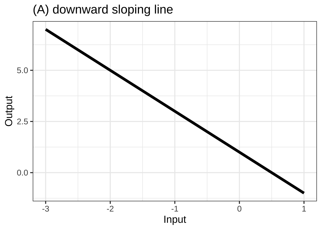
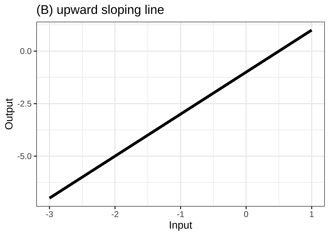
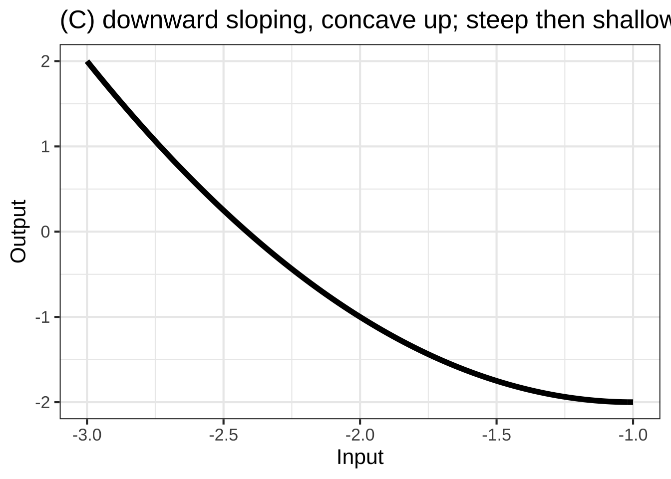
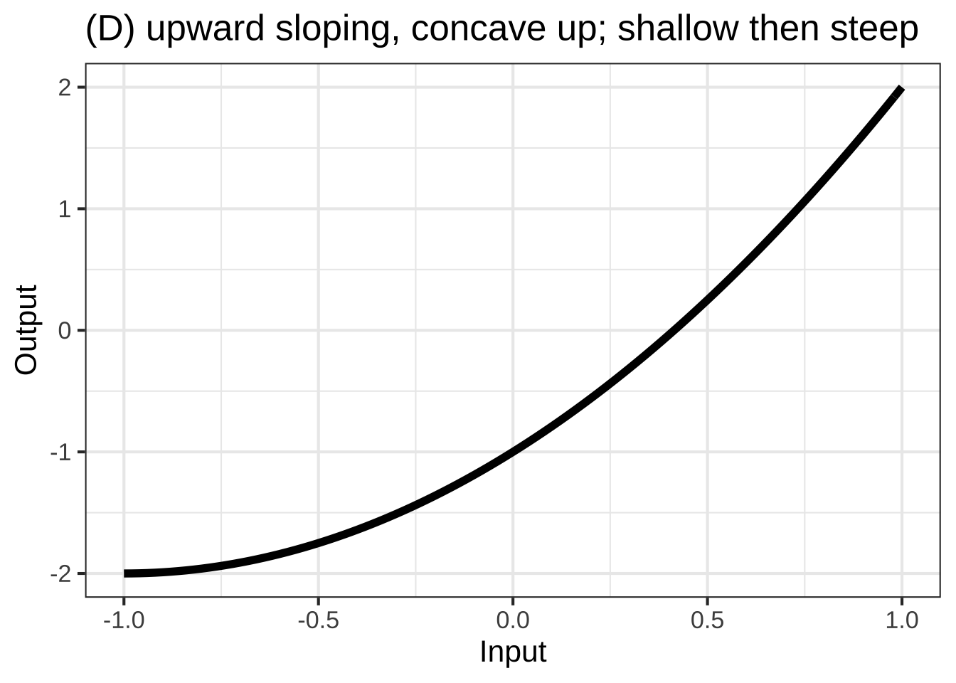
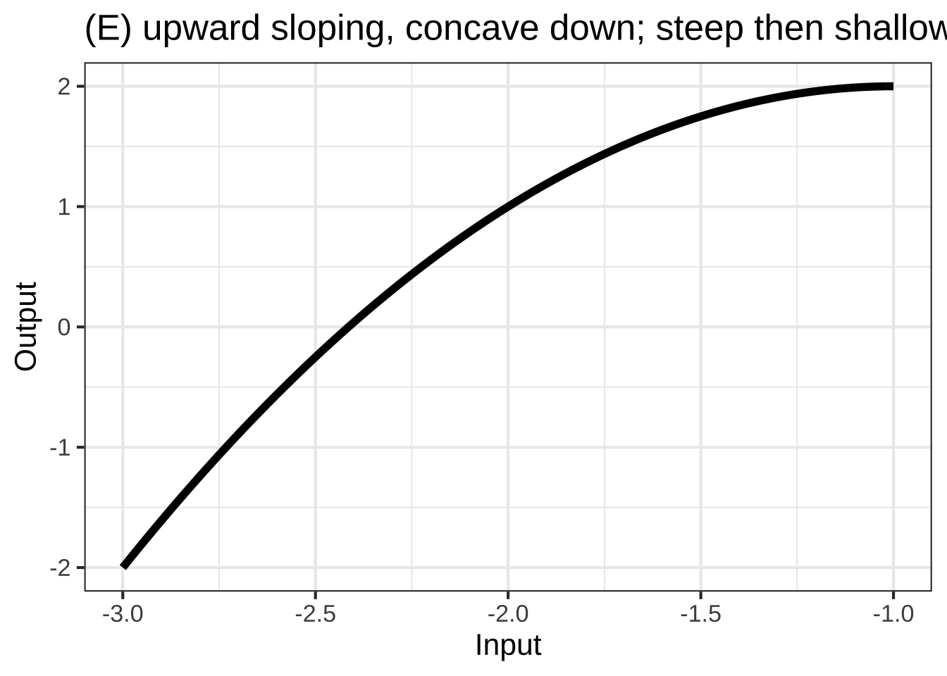
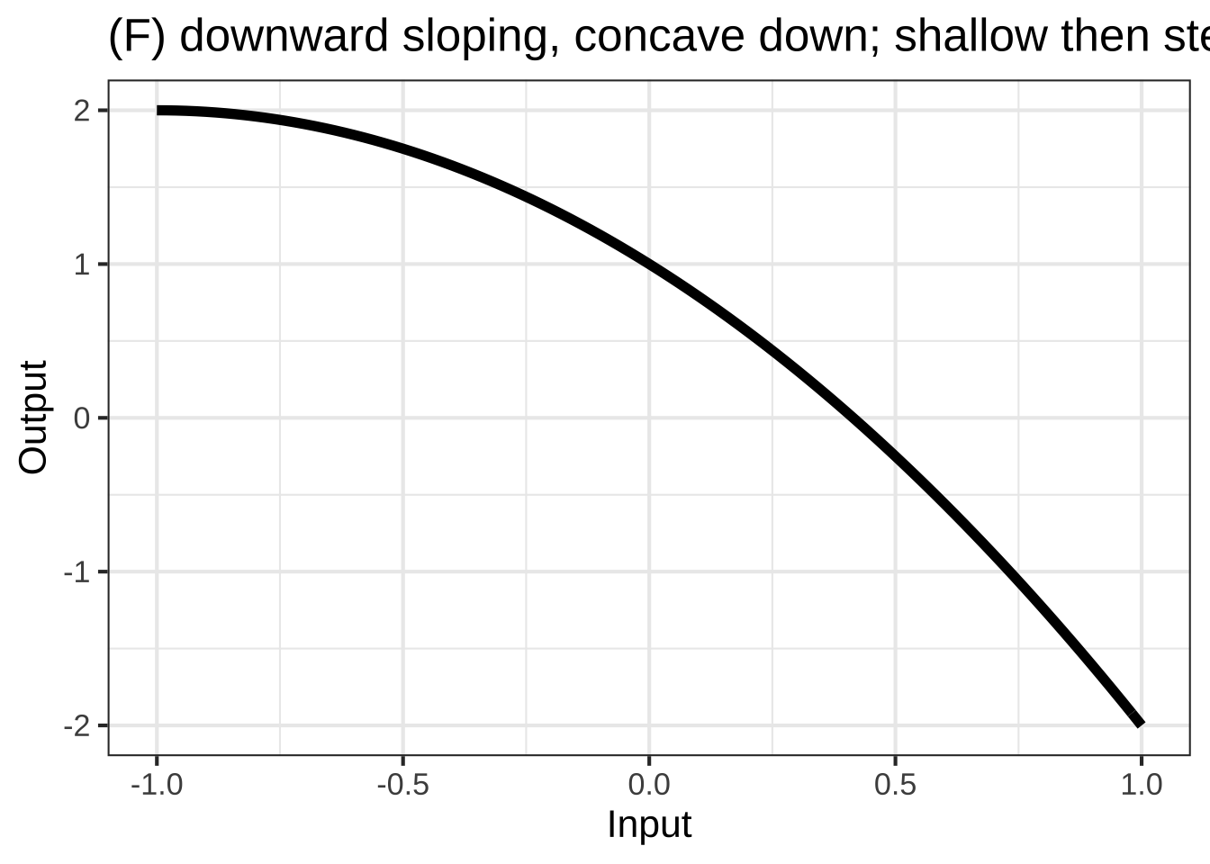
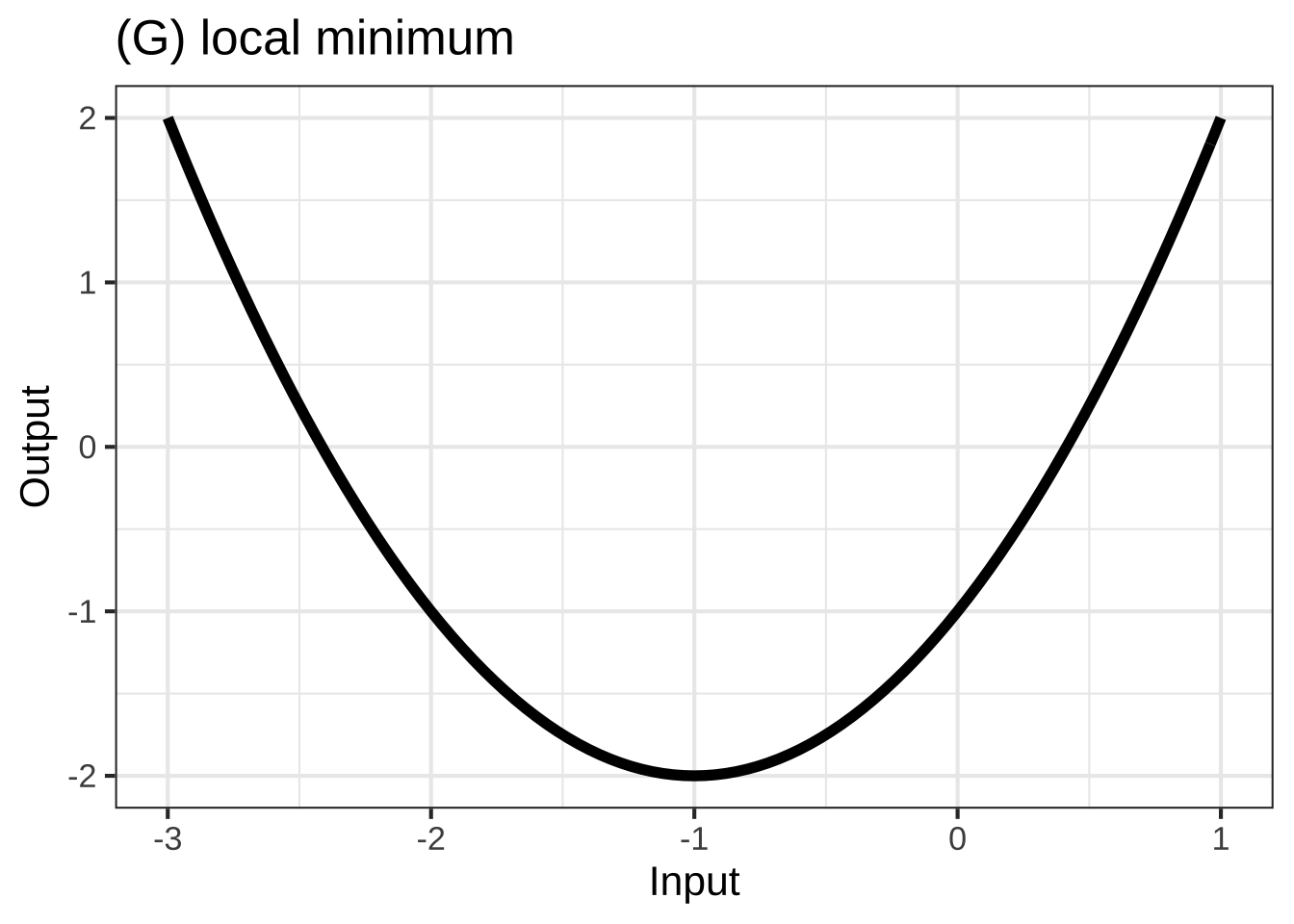
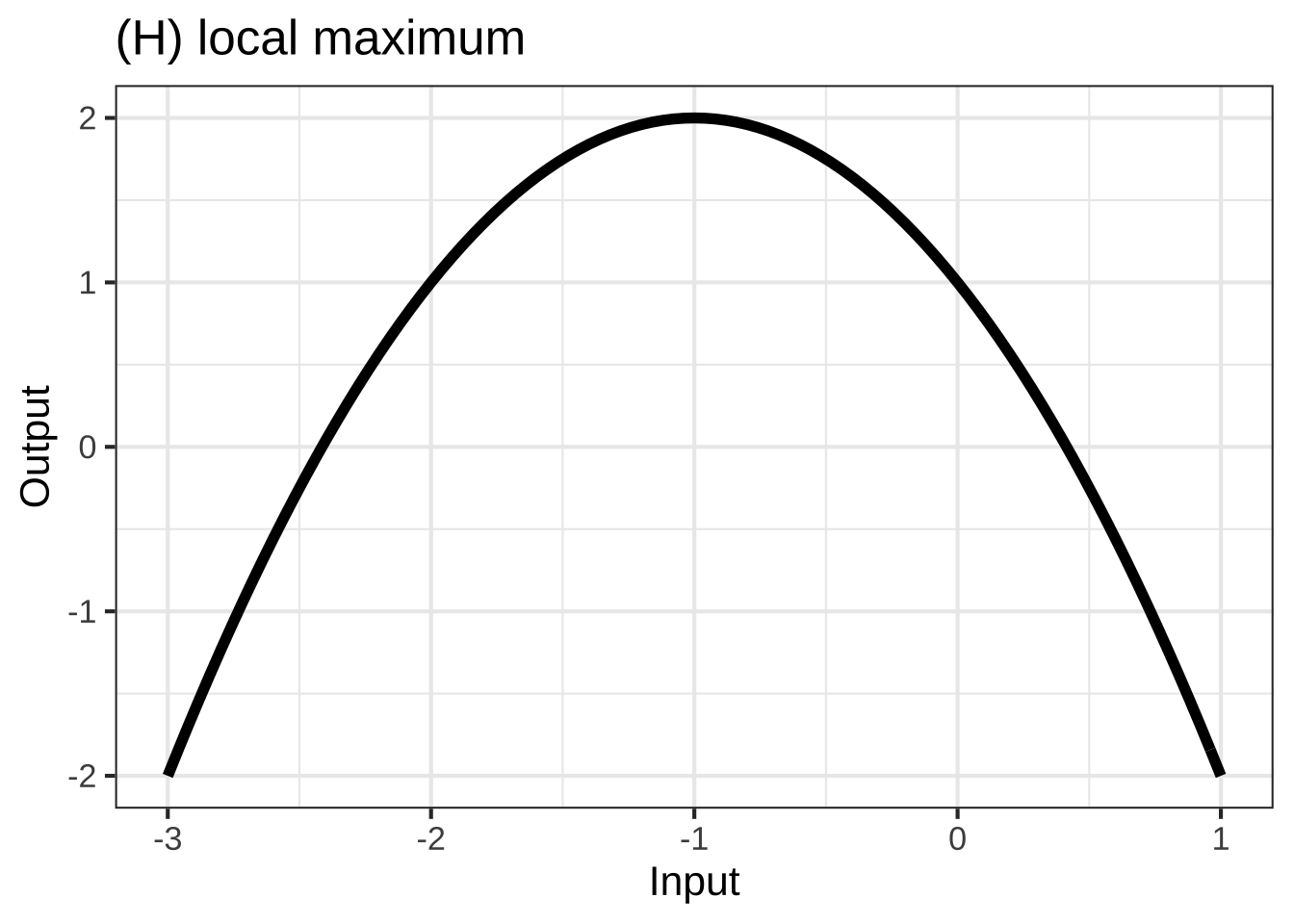
To choose among these shapes, consider your modeling context: 2795

• is the relationship positive (slopes up) or negative (slopes down)
• is the relationship monotonic or not
• is the relationship concave up, concave down, or neither

Some examples, scenarios where the modeler knows about the derivative and concavity of the relationship being modeled. It’s often the case that your knowledge of the system comes in this form. 2800

• The incidence of an out-of-control epidemic versus time is concave up, but shallow-then-steep. As the epidemic is brought under control, the decline is steep-then-shallow and concave up. Over the whole course of an epidemic, there is a maximum incidence. Experience shows that epidemics can have a phase where incidence reaches a local minimum: a decline as people practice social distancing followed by an increase as people become complacent. 2805

• How many minutes can you run as a function of speed? Concave down and shallow-then-steep; you wear out faster if you run at high speed. How far can you walk as a function of time? Steep-then-shallow and concave down; your pace slows as you get tired.

• How does the stew taste as a function of saltiness. The taste improves as the amount of salt increases … up to a point. Too much salt and the stew is unpalatable.

• The temperature of cooling water or the emission of radioactivity as functions of time are concave up and steep-then-shallow. 2810

• How much fuel is consumed by an aircraft as a function of distance? For long flights the function is concave up and shallow-then-steep; fuel use increases with distance, but the amount of fuel you have to carry also increases with distance and heavy aircraft use more fuel per mile.

• In micro-economic theory there are production functions that describe how much of a good is produced at any given price, and demand functions that describe how much of the good will be purchased as a function of price. 2815

  • As a rule, production increases with price and demand decreases with price. In the short term, production functions tend to be concave down, since it’s hard to squeeze increased production out of existing facilities.
    
  • For demand in the short term, functions will be concave up when there is some group of consumers who have no other choice than to buy the product. An example is the consumption of gasoline versus price: it’s hard in the short term to find another way to get to work. In the long term, consumption functions can be concave down as consumers find alternatives to the high-priced good. For example, high prices for gasoline may, in the long term, prompt a switch to more efficient cars, hybrids, or electric vehicles. This will push demand down steeply. 2820

2825

25.2 Low-order polynomials

There is a simple, familiar functional form that, by selecting parameters appropriately, can take on each of the eight simple shapes: the second-order polynomial. \[g(x) \equiv a + b x + c x^2\] As you know, the graph of \(g(x)\) is a parabola.

• The parabola opens upward if \(0 < c\). That’s the shape of a local minimum.
• The parabola opens downward if \(c < 0\). That’s the shape of a local maximum

Consider what happens if \(c = 0\). The function becomes simply \(a + bx\), the straight-line function.

• When \(0 < b\) the line slopes upward.
• When \(b < 0\) the line slopes downward.

With the appropriate choice of parameters, the form \(a + bx + cx^2\) is capable of representing four of the eight simple shapes. What about the remaining four? This is where the idea of local becomes important. Those remaining four shapes are the sides of parabolas, as in Figure ??. 2830

## Warning in validate_domain(domain, free_args): Missing domain names: x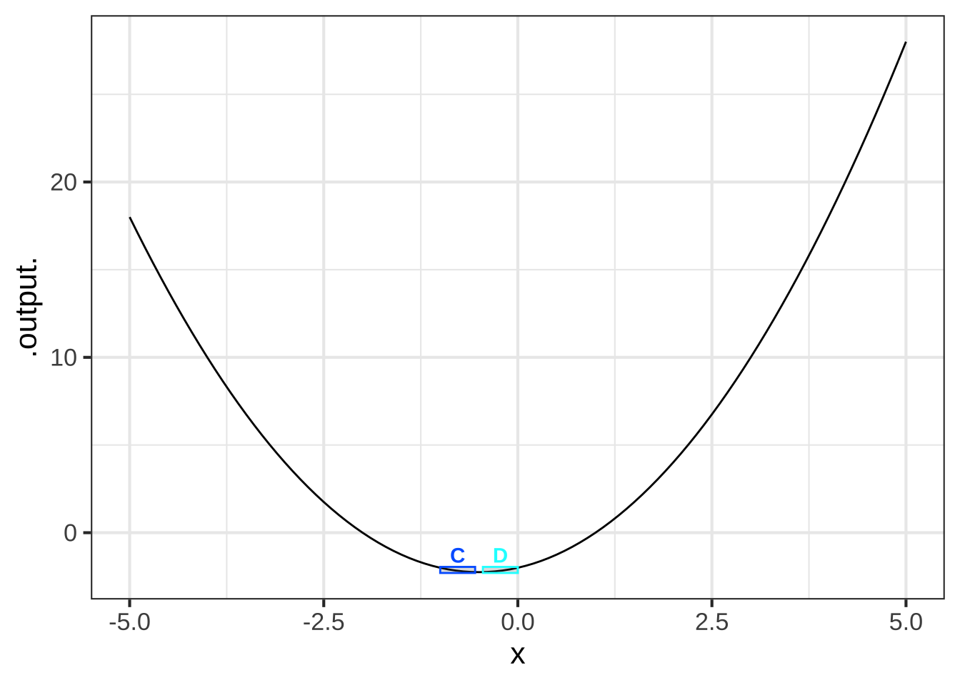

Figure 25.2: Four of the eight simple shapes correspond to the sides of the parabola. The labels refer to the graphs in Figure 25.1.

## Warning in validate_domain(domain, free_args): Missing domain names: x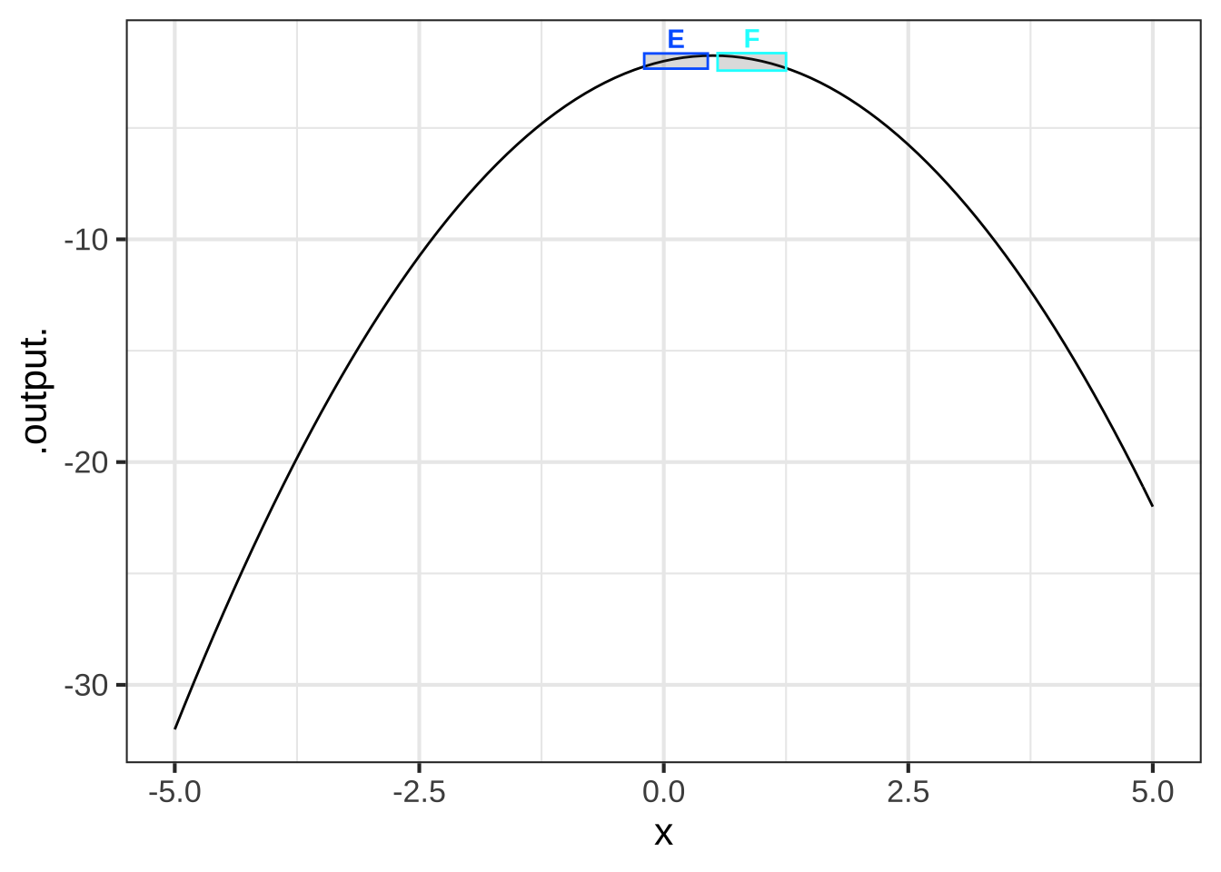

Figure 25.3: Four of the eight simple shapes correspond to the sides of the parabola. The labels refer to the graphs in Figure 25.1.

25.3 The low-order polynomial with two inputs

For functions with two inputs, the low-order polynomial approximation looks like this:

\[g(x, y) \equiv a_0 + a_x x + a_y y + a_{xy} x y + a_{yy} y^2 + a_{xx} x^2\] In reading this form, note the system being used to name the polynomial’s coefficients. First, we’ve used \(a\) as the root name of all the coefficients. Sometimes we might want to compare two or more low-order polynomials, so it’s convenient to be able to use \(a\) for one, \(b\) for another, and so on. 2835

The subscripts on the coefficients describes exactly which term in the polynomial involves each coefficient. For instance, the \(a_{yy}\) coefficient applies to the \(y^2\) term, while \(a_x\) applies to the \(x\) term. 2840

Each of \(a_0, a_x,\) \(a_y,\) \(a_{xy}, a_{yy}\), and \(a_{xx}\) will, in the final model, be a constant quantity. Don’t be confused by the use of \(x\) or \(y\) in the name of the coefficients. Each coefficient is a constant and not a function of the inputs. Often, your prior knowledge of the system being modeled will tell you something about one or more of the coefficients, for example, whether it is positive or negative. Finding a precise value is often based on quantitative data about the system. 2845

It helps to have different names for the various terms. It’s not too bad to say something like, “the \(a_{xy}\) term.” (Pronounciation: “a sub x y” or “a x y”) But the proper names are: linear terms, quadratic terms, and interaction term. And a shout out to \(a_0\), the constant term. 2850

\[g(x, y) \equiv a_0 + \underbrace{a_x x + a_y y}_\text{linear terms} \ \ \ + \underbrace{a_{xy} x y}_\text{interaction term} +\ \ \ \underbrace{a_{yy} y^2 + a_{xx} x^2}_\text{quadratic terms}\]

## Warning in validate_domain(domain, free_args): Using -5 to 5 in domain for
## missing domain names.

## Warning in validate_domain(domain, free_args): Missing domain names: x, y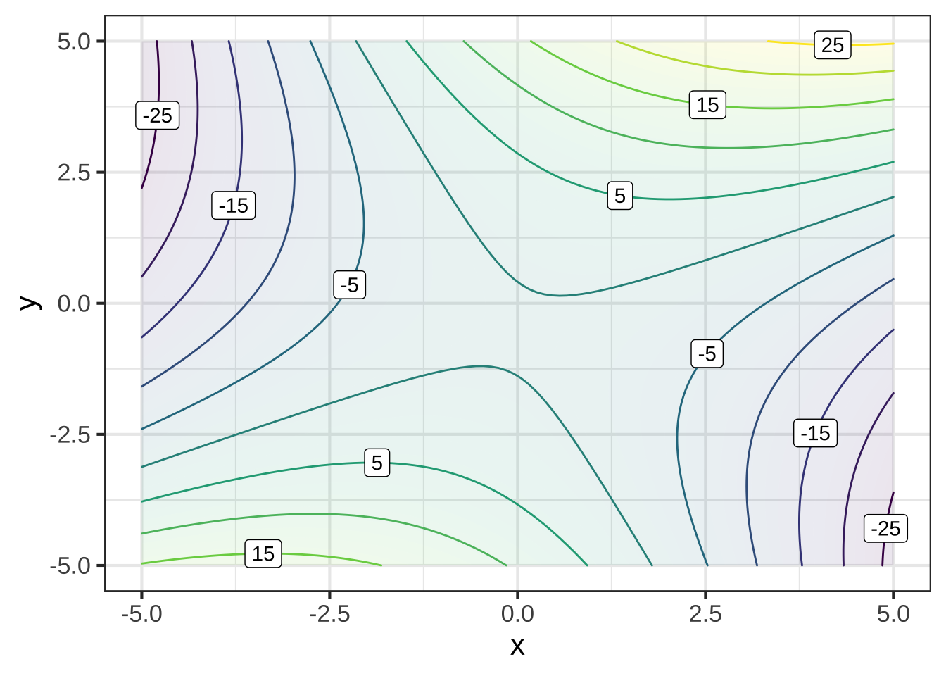

Figure 25.4: A saddle

Figure 25.4: A saddle

If you’re like many people, you find it harder to walk uphill than down, and find it takes more out of you to walk longer distances than shorter. Let’s build a model of this, using nothing more than your intuition and the method of low-order polynomial approximations.

Let’s call the map distance walked \(d\). (“Map distance” is the horizontal change in position, disregarding vertical changes.) The steepness of the hill will be the “grade” \(g\), which is measured as the horizontal distance covered divided by the vertical climb. If you’re going downhill, the grade is negative.

The key ingredient in the model: We’ll measure the “difficulty” or “exertion” to walking as the energy consumed during the walk: \(E(d, g)\).

Some assumptions about walking and energy consumed:

1. If you don’t walk, you consume zero energy walking.
2. The energy consumed should be proportional to the length of the walk. This is an assumption, and is probably valid, only for walks of short to medium distances, as opposed to forced marches over tens of miles.

We’ll start with the full 2nd-order polynomial in two variables, and then seek to eliminate terms that aren’t needed.

\[E_{big}(d, g) \equiv a_0 + a_d\, d + a_g\, g + a_{dg}\, d\, g + a_{dd}\,d^2 + a_{gg}\,g^2\] According to assumption (1), when \(E(d=0, g) = 0\). Of course, if you are walking zero distance, it doesn’t matter what the grade is; the energy consumed is still zero.

Consequently, we know that all terms that don’t include a \(d\) should go away. This leaves us with

\[E_{medium}(d, g) \equiv a_d\, d + a_{dg}\, d\, g + a_{dd}\,d^2 = d \left[\strut a_d + a_{dg}\, g + a_{dd}\,d\right]\] Assumption (2) says that energy consumed is proportional to \(d\). The multiplier on \(d\) in \(E_{medium}()\) is \(\left[\strut a_d + a_{dg}\, g + a_{dd}\,d\right]\) which is itself a function of \(d\). A proportional relationship implies a multiplier that doesn’t depend on the quantity itself. This means that \(a_{dd} = 0\).

This leaves us with a very simple model: \[E(d, g) \equiv \left[\strut a_1 + a_2\, g\right]\, d\] where we have simplified the labeling on the coefficients since there are only two in the model.

Perhaps assumption (2) is mis-placed and that the energy consumed per unit distance in a walk increases with the length of the walk. If so, we would need to return to the question of \(a_{dd}\). This is typical of the modeling cycle. Trying to be economical with model terms highlights the question of which terms are so small they can be ignored.

Example 25.1 In selecting cadets for pilot training, two criteria are the cadet’s demonstrated flying aptitude and the leadership potential of the cadet. Let’s assume that the overall merit \(M\) of a candidate is a function of flying aptitude \(F\) and leadership potential \(L\).

Currently, the merit score is a simple function of the \(F\) and \(L\) scores: \[M_{current}(F, L) \equiv F + L\]

The general in charge of the training program is not satisfied with the current merit function. “I’m getting too many cadets who are great leaders but poor pilots, and too many pilot hot-shots who are not good leaders. I would rather have an good pilot who is a good leader than have a great pilot who is a poor leader or a poor pilot who is a great leader.” (You might reasonably agree or disagree with this point of view, but the general is in charge.)

The general has tasked you to revise the formula to better match her views about the balance betwen flying ability and leadership potential.

How should you go about constructing \(M_{improved}(F, L)\)?

You recognize that \(F + L\) is a low-order polynomial: just the linear terms are present without a constant or interaction term or quadratic terms. Low-order polynomials are a good way to approximate any formula locally, so you have decided to follow that route.

Quadratic terms are appropriate when a model needs to feature a locally optimal level of the of the inputs. But it will never be the case that a lower flying score will be more favored than a higher score, and the same thing for the leadership score. So your model doesn’t need quadratic terms.

That leaves the interaction term as the way forward. The low-order polynomial model will be \[M_{improved}(F, L) \equiv d_0 + F + L + d_{FL} FL\] Should \(d_{FL}\) be positive or negative?

Imagine a cadet Drew with acceptable and equal F and L scores. Another cadet, Blake, has scores that are \(F+\epsilon\) and \(L-\epsilon\), where \(\epsilon\) might be positive or negative. Under the original formula for merit, Drew and Blake have equal merit. Under the new criteria, Drew should have a higher merit than Blake. In other words: \[M_{improved}(F, L) - M_{improved}(F+\epsilon, L-\epsilon) > 0\]

Replace \(M_{improved}(F, L)\) with the low-order polynomial approximation given earlier. \[\underbrace{d_0 + F + L + d_{FL} FL}_{M_{improved}(F, L)} - \underbrace{\left[{\large\strut} d_0 + \left[ F + \epsilon\right] + \left[ L - \epsilon\right] + d_{FL} (FL -\epsilon L + \epsilon F - \epsilon^2)\right]}_{M_{improved}(F+\epsilon, L-\epsilon)} > 0\] Collecting and cancelling terms in the above gives \[- d_{FL}(\epsilon(F-L) + \epsilon^2) > 0\] Since \(F\) and \(L\) were assumed equal, this results in \[M_{improved}(F, L) - M_{improved}(F+\epsilon, L-\epsilon) = d_{FL}\, \epsilon^2 > 0\] Thus, \(d_{FL}\) will have to be positive.

25.4 Finding coefficients from data

Low-order polynomials are often used for constructing functions from data. In this section, I’ll demonstrate briefly how this can be done. The full theory will be introduced in Block 5 of this text.

The data I’ll use for the demonstration is a set of physical measurements of height, weight, abdominal circumference, etc. on 252 human subjects. These are contained in the Body_fat data frame, shown below.

One of the variables records the body-fat percentage, that is, the fraction of the body’s mass that is fat. This is thought to be an indicator of fitness and health, but it is extremely hard to measure and involves weighing the person when they are fully submerged in water. This difficulty motivates the development of a method to approximation body-fat percentage from other, easier to make measurements such as height, weight, and so on.

For the purpose of this demonstration, we’ll build a local polynomial model of body-fat percentage as a function of height (in inches) and weight (in pounds).

The polynomial we choose will omit the quadratic terms. It will contain the constant, linear, and interaction terms only. That is \[\text{body.fat}(h, w) \equiv c_0 + c_h h + c_w w + c_{hw} h w\] The process of finding the best coefficients in the polynomial is called linear regression. Without going into the details, we’ll use linear regression to build the body-fat model and then display the model function as a contour plot.

mod <- lm(bodyfat ~ height + weight + height*weight,
          data = math141Z::Body_fat)
body_fat_fun <- makeFun(mod)
contour_plot(body_fat_fun(height, weight) ~ height + weight,
             domain(weight=c(100, 250), height = c(60, 80))) %>%
  gf_labs(title = "Body fat percentage")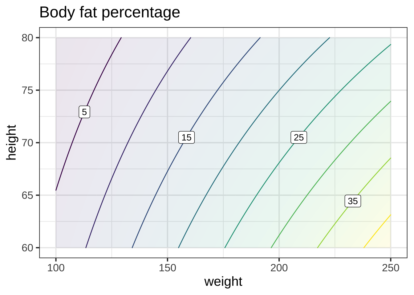

Figure 25.5: A low order polynomial model of body fat percentage as a function of height (inches) and weight (lbs).

That we can build such a model doesn’t mean that it’s useful for anything. In Block 5 of the text we’ll return to the question of how well a model constructed from data represents the real-world relationships that the model attempts to describe.

25.5 Exercises

Exercise 25.02: ckslw

Consider the model presented in Section 25.3 about energy expenditure walking distance \(d\) on a grade \(g\): \[E(d,g) = (a_0 + a_1 g)d\] where \(d\) is the (horizontal equivalent) of the distance walked and \(g\) is the grade of the slope (that is, rise over run).

We want \(E\) to be measured in Joules which has dimension M L\(^2\) T\(^{-2}\). Of course, the dimension of \(d\) is L, that is \([d] = \text{L}\).

What is the dimension of the parameter $$a_0$$? 



( )  dimensionless
( )  $$L/T^2$$
( )  $$T/L^2$$
( )  $$M/T^2$$
(x )  $$M L/T^2$$
( )  $$M/L^2$$
( )  $$M/(L^2 T^2)$$
( )  $$M L^2 / T^2$$

[[Nice!]]

What is the dimension of $$g$$? (Hint: $$g$$ is the ratio of vertical to horizontal distance covered.) 



(x )  dimensionless
( )  $$L/T^2$$
( )  $$T/L^2$$
( )  $$M/T^2$$
( )  $$M L/T^2$$
( )  $$M/L^2$$
( )  $$M/(L^2 T^2)$$
( )  $$M L^2 / T^2$$

[[Excellent!]]

What is the dimension of the parameter $$a_1$$? 



( )  dimensionless
( )  $$L/T^2$$
( )  $$T/L^2$$
( )  $$M/T^2$$
(x )  $$M L/T^2$$
( )  $$M/L^2$$
( )  $$M/(L^2 T^2)$$
( )  $$M L^2 / T^2$$

[[Nice!]]

Exercise 25.04: ikdlx

Suppose we describe the spread of an infection in terms of three variables:

• \(N\) infection rate with respect to time: the number of new infections per day
• \(I\) the current number of people who are infectious, that is, currently capable of spreading the infection
• \(S\) the number of people who are susceptible, that is, currently capable of becoming infectious if exposed to the infection.

All three of these variables are functions of time. News reports in 2020 routinely such as the one below gave the graph of \(N\) versus time for Covid-19.

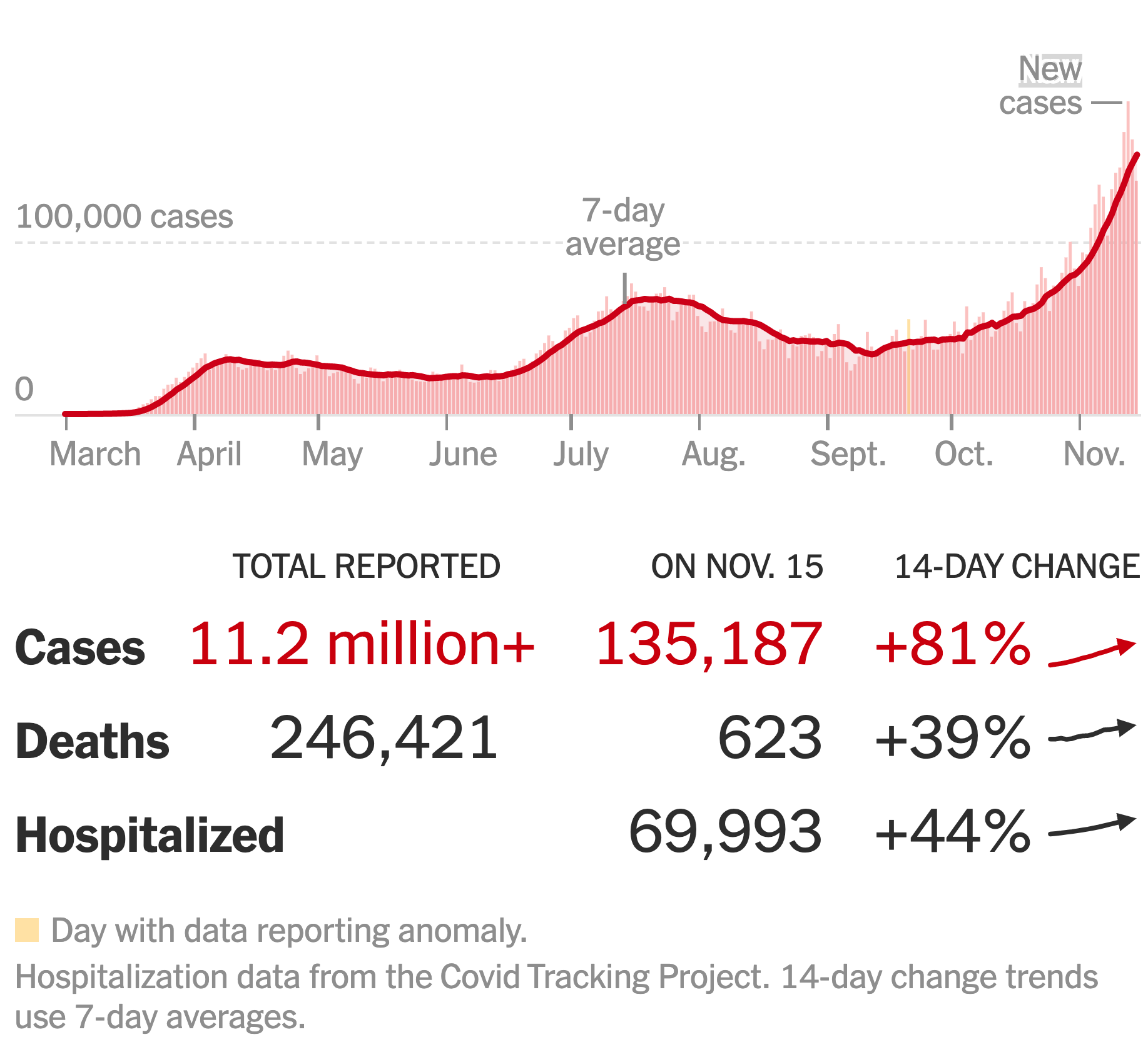
On November 15, 2020, \(N\) was 135,187 people per day. (This is the number of positive tests. The true value of \(N\) was, based on later information, 5-10 times greater.) The news reports don’t usually report \(S\) on a day-by-day basis.

But a basic strategy in modeling with calculus is to take a snapshot: Given \(I\) and \(S\) today, what is a model of \(N\) for today. (Next semester, we’ll study “differential equations,” which provide a way of assembling from the snapshot model what the time course of the pandemic will look like.)

The low-order polynomial for \(N(S, I)\) is \[N(S,I) = a_0 + a_1 S + a_2 I + a_{12} I S.\] We don’t include quadratic terms because there is no local maximum in \(N(S, I)\)—common sense suggests that \(\partial_S N() \geq 0\) and \(\partial_I N() \geq 0\), whereas a local maximum requires at least one of these derivatives to be negative near the max.

Your job is to figure out which, if any, terms can be safely deleted from the low-order polynomial. A good way to approach this is to figure out, using common sense, what \(N\) would be for either \(S=0\) or \(I=0\). (Note that the previous is not restricted to \(S = I = 0\). Only one of them needs to be zero to produce the relevant result.)

Which of these is a sufficiently complete low-order polynomial given the behavior of $$N$$ at $$S=0$$ or $$I=0$$? 



( )  $$N(S,I) = a_0 + a_1 S + a_2 I + a_{12} I S$$
( )  $$N(S,I) = a_0 + a_1 S + a_2 I$$
( )  $$N(S,I) = a_1 S + a_2 I + a_{12} I S$$
( )  $$N(S,I) = a_2 I + a_{12} I S$$
( )  $$N(S,I) = a_1 S + a_{12} I S$$
(x )  $$N(S,I) = a_{12} I S$$
( )  $$N(S,I) = a_1 S + a_2 I$$

[[Correct.]]