30 Integrals step-by-step
The setting for anti-differentiation (and it’s close cousin, integration) is that we have a function \(F(t)\) which we do not yet know, but we do have access to some information about it: its slope as a function of time \(f(t) \equiv \partial_t F(t)\) and, perhaps, its value \(F(t_0)\) at some definite input value.
Chapter 28 showed some ways to visualize the construction of an \(F(t)\) by accumulating short segments of slope. The idea is that we know \(f(t)\) which tells us, at any instant, the slope of \(F(t)\). So, in drawing a graph of \(F(t)\), we put our pen to paper at some input value \(t_0\) and then move forward in \(t\), setting the instantaneous slope of our curve according to \(f(t)\).
In Chapter 29, we dealt with one of the limitations of finding \(F(t)\) by anti-differentiation of \(f(t)\); the anti-derivative is not unique. This is because to start drawing \(F(t)\) we need pick a \(t_0\) and an initial value of \(F(t_0)\). If we had picked a a different starting point \(t_1\) or a different initial value \(F(t_1)\), the new curve would be different than the one drawn through \((t_0, F(t_0))\), although it would have the same shape, just shifted up or down according to our choice. We summarize this situation algebraically by writing \[\int f(t) dt = F(t) + C\ ,\] where \(C\) is the constant of integration, that is, the vertical shift of the curve.
The non-uniqueness of \(F(t)\) does not invalidate its usefulness. In particular, the quantity \(F(b) - F(a)\), will be the same regardless of which starting point we used to draw \(F(t)\). We have two names for \(F(b) - F(a)\)
- The net change in \(F()\) from \(a\) to \(b\).
- The definite integral of \(f()\) from \(a\) to \(b\), written \(\int_a^b f(t) dt\).
These two things, the net change and the definite integral, are really one and the same, a fact we describe by writing \[\int_a^b f(t) dt = F(b) - F(a)\].
In this chapter, we’ll introduce a simple numerical method for calculating from \(f()\) the net change/definite integral. This will be a matter of trivial but tedious arithmetic: adding up lots of little bits of \(f(t)\). Later, in Chapter 31, we’ll see how to avoid the tedious arithmetic by use of algebraic, symbolic transformations. This symbolic approach has great advantages, and is the dominant method of anti-differentiation found in college-level science textbooks. However, there are many common \(f(t)\) for which the symbolic approach is not possible, whereas the numerical method works for any \(f(t)\). Even more important, the numerical technique has a simple natural extension to some commonly encountered accumulation problems that look superficially like they can be solved by anti-differentiation but rarely can be in practice. We’ll meet one such problem and solve it numerically, but a broad approach to the topic, called dynamics or differential equations, will have to wait until Block 6.
30.1 Euler method
The starting point for this method is the definition of the derivative of \(F(t)\). Reaching back to Chapter @ref{fun-slopes},
\[\partial_t F(t) \equiv \lim_{h\rightarrow 0} \frac{F(t+h) - F(t)}{h}\] To translate this into a numerical method for computing \(F(t)\), let’s write things a little differently.
- First, since the problem setting is that we don’t (yet) know \(F(t)\), let’s refer to things we do know. In particular, we know \(f(t) = \partial_t F(t)\).
- Again, recognizing that we don’t yet know \(F(t)\), let’s re-write the expression using something that we do know: \(F(t_0)\). Stated more precisely, \(F(t_0)\) is something we get to make up to suit our convenience. (A common choice is \(F(t_0)=0\).)
- Let’s replace the symbol \(h\) with the symbol \(dt\). Both of them mean “a little bit of” and \(dt\) makes explicit that we mean “a little bit of \(t\).”
- We’ll substitute the limit \(\lim_{h\rightarrow 0}\) with an understanding that \(dt\) will be something “small.” How small? We’ll deal with that question when we have to tools to answer it.
With these changes, we have \[f(t_0) = \frac{F(t_0+dt) - F(t_0)}{dt}\ .\] The one quantity in this relationship that we do not yet know is \(F(t_0 + dt)\). So re-arrange the equation so that we can calculate the unknown in terms of the known. \[F(t_0 + dt) = F(t_0) + dt\, f(t_0)\ .\]
Example 30.1 Let’s consider finding the anti-derivative of \(\dnorm()\), that is, \(\int_0^t \dnorm(x) dx\). In one sense, you already know the answer, since \(\partial_x \pnorm(x) = \dnorm(x)\). In reality, however, we know \(\pnorm()\) only because it has been numerically constructed by integrating \(\dnorm()\). The \(\pnorm()\) function is so important that the numerically constructed answer has been memorized by software
30.3 Exercises
Exercise 30.02:  ady5Fh
The output of a function, being a quantity, has dimension and units. Suppose the dimension of the output of a function \(v(t)\) is \(L/T\), for instance, meters-per-second.
The anti-derivative function \(V(t) \equiv \int v(t) dt\) will also have dimension and units.
Recall that in constructing the anti-derivative using the Euler method, we multiply the values of \(v(t)\) times some small increment in the input, \(h\). Therefore the dimension of the output of \(V(t)\) will be \([v(t)] [t]\). So if \([v(t)] = L/T\), the dimension \([V(t)] [t] = L T/T = L\). Units for such a dimension would be, for instance, meters. This makes sense, since if you accumulate velocity (meters-per-sec) over an interval of time (sec) you end up with the distance travelled (meters).
Suppose you know the acceleration \(a(t)\) of an object as a function of time. The dimension of acceleration is \(L/T^2\).
askMC(
  "What is the dimension of $$\\int a(t) dt\\ \\text{?}$$",
  "$L/T^3$", "$L$", "$LT$", "+$L/T$+", "$LT^2$"
)
What is the dimension of $$$\int a(t) dt\ \text{?}$$$
( ) $$L/T^3$$
( ) $$L$$
( ) $$LT$$
(x ) $$L/T$$
( ) $$LT^2$$
[[Correct.]]
Suppose you know the power consumed by an appliance \(p(t)\) as a function of time. Typically appliances have a cycle and use different amounts of power during different parts of the cycle. (Think of a clothes washer.)
askMC(
  "What will be the dimension of $\\int p(t) dt\\ \\text{?}$",
  "+energy+", "force", "acceleration", "length"
)
What will be the dimension of $$\int p(t) dt\ \text{?}$$
(x ) energy
( ) force
( ) acceleration
( ) length
[[Excellent!]]
Exercise 30.04: CCwWGB
In this activity, you are going to use the “Graph-antiD” web app which enables you to visualize the anti-derivative function in terms of areas. To use the app, click-drag-and-release to mark part of the domain of the function being displayed.
Add a picture of the app and a link to it.
To answer these questions correctly, you must set the “Shape of function” box to 864.
askMC(
  "A. From the graph, roughly estimate $$\\int_0^3 f(t)dt$$ Choose the closest numerical value from the following. You could use either graph for this caclulation, but $F(t)$ will be simpler algebra.",
  -46, -26, "0"="F(t) has a net change over the interval", "3"="there is more stock at F(3) than F(0)", "19"="there is more stock at F(3) than F(0)", "26"="F(t) at the right end of the interval is lower than at the left end", right_one = -26,
  random_answer_order = FALSE
)
A. From the graph, roughly estimate $$$\int_0^3 f(t)dt$$$ Choose the closest numerical value from the following. You could use either graph for this caclulation, but $$F(t)$$ will be simpler algebra. ( ) -46 (x ) -26 ( ) 0 ( ) 3 ( ) 19 ( ) 26 [[Good.]]
askMC(
  "B. In order to construct the anti-derivative whose value at time $t=-3$ will be zero, what constant of integration $C$ should you **add** to the $F(t)$ shown.",
  "-120"= "Would adding this to F(-3) be equal to 0?", "-80"= "Would adding this to F(-3) be equal to 0?", "-50"= "Would adding this to F(-3) be equal to 0?", "0"= "Would adding this to F(-3) be equal to 0?", "50" = "Would adding this to F(-3) be equal to 0?",
  "80" = "Are you sure you have the sign right?",
  "120" = "Would adding this to F(-3) be equal to 0?",
  right_one = -80,
  random_answer_order = FALSE
)
B. In order to construct the anti-derivative whose value at time $$t=-3$$ will be zero, what constant of integration $$C$$ should you **add** to the $$F(t)$$ shown. ( ) -120 (x ) -80 ( ) -50 ( ) 0 ( ) 50 ( ) 80 ( ) 120 [[Would adding this to F(-3) be equal to 0?]]
askMC(
  "C. Examining the stock at time $t=0$, you observe that there are 40 units. Roughly how much stock will there be at $t=5$?",
  "-25" = "Did you shift the curve in the right direction?", "-15" = "That would be the answer if there had been 0 units of stock at time $t=0$.","0"="Imagine F(t) being shifted by the difference of 40 and F(0)", "15"="Imagine F(t) being shifted by the difference of 40 and F(0)",  25, right_one=25,
  random_answer_order = FALSE
)
C. Examining the stock at time $$t=0$$, you observe that there are 40 units. Roughly how much stock will there be at $$t=5$$? ( ) -25 ( ) -15 ( ) 0 ( ) 15 (x ) 25 [[Excellent!]]
askMC(
  "D. You start with a stock of 100 units at time $t = -2$. At roughly what time $t$ will the stock be half of this?",
  "-1.2"="$F(t)$-$F(a)$=50, what is the value of a?", -0.3, "0.5"="$F(t)$-$F(a)$=50, what is the value of a?", "1.2"="$F(t)$-$F(a)$=50, what is the value of a?", "1.8"="$F(t)$-$F(a)$=50, what is the value of a?",
  "The stock will never fall so low.",
  right_one = -0.3,
  random_answer_order = FALSE
)
D. You start with a stock of 100 units at time $$t = -2$$. At roughly what time $$t$$ will the stock be half of this? ( ) -1.2 (x ) -0.3 ( ) 0.5 ( ) 1.2 ( ) 1.8 ( ) The stock will never fall so low. [[Correct.]]
askMC(
  "E. Your stock finally runs out at time $t=2.5$. When did you have 120 units in stock?",
  "+$t=-4$+", "$t=-3$"="This uses a similiar approach to the last question.", "$t=0$"="This uses a similiar approach to the last question.",
  "There was never such a time."
)
E. Your stock finally runs out at time $$t=2.5$$. When did you have 120 units in stock? (x ) $$t=-4$$ ( ) $$t=-3$$ ( ) $$t=0$$ ( ) There was never such a time. [[Nice!]]
askMC(
  "F. After decreasing for a long time, the stock finally starts to increase from about $t=2.5$ onward. What about $f(t=2.5)$ tells you that $F(t=2.5)$ is increasing?",
  "The derivative is at a minimum."="Does this mean $F(t)$ must be increasing?",
  "The derivative is negative"="Does this mean $F(t)$ must be increasing?",
  "The derivative is near zero." = "Kind of. For the stock $F(t)$ to increase, what has to be true of the derivative at that instant.",
  "+The derivative becomes positive and stays positive.+",
  "The derivative is at a maximum."="Does this mean $F(t)$ must be increasing?",
  random_answer_order = FALSE
)
F. After decreasing for a long time, the stock finally starts to increase from about $$t=2.5$$ onward. What about $$f(t=2.5)$$ tells you that $$F(t=2.5)$$ is increasing? ( ) The derivative is at a minimum. ( ) The derivative is negative ( ) The derivative is near zero. (x ) The derivative becomes positive and stays positive. ( ) The derivative is at a maximum. [[Right!]]
askMC(
  "G. Find the argmin $t^\\star$ of $f(t)$ and note the sign of $f(t^\\star).$  What does this tell you about $F(t^\\star)$.",
  "$t^\\star$ is also the argmin of $F()$."="look at the corresponding point on $F(t)$.",
  "+$F(t^\\star)$ is decreasing at its steepest rate.+",
  "$F(t^\\star)$ is increasing at it's slowest rate."="look at the corresponding point on $F(t)$.",
  "$F(t^\\star)$ is increasing at its steepest rate."="look at the corresponding point on $F(t)$.",
  "$t^\\star$ is the argmax of $F()$"="look at the corresponding point on $F(t)$."
)
G. Find the argmin $$t^\star$$ of $$f(t)$$ and note the sign of $$f(t^\star).$$ What does this tell you about $$F(t^\star)$$. ( ) $$t^\star$$ is also the argmin of $$F()$$. (x ) $$F(t^\star)$$ is decreasing at its steepest rate. ( ) $$F(t^\star)$$ is increasing at it's slowest rate. ( ) $$F(t^\star)$$ is increasing at its steepest rate. ( ) $$t^\star$$ is the argmax of $$F()$$ [[Nice!]]
askMC(
  "H. What is the average flow into stock over the period $-5 \\leq t \\leq 1$. (If the flow is *outward from stock*, that's the same as a negative inward flow.)",
  -30, -20, "0" = "But you can see that the stock is diminishing steadily during $-5 \\leq t \\leq 1$, so how could the average flow be zero.", "10", right_one = -20,
  random_answer_order = FALSE
)
H. What is the average flow into stock over the period $$-5 \leq t \leq 1$$. (If the flow is *outward from stock*, that's the same as a negative inward flow.) ( ) -30 (x ) -20 ( ) 0 ( ) 10 [[Nice!]]
askMC(
  "I. Which of the following is an interval when the average flow is approximately zero?",
  "$-1.3 \\leq t \\leq 1.1$"="The area appears to be negative.",
  "+$0.8 \\leq t \\leq 5$+",
  "$-5 \\leq t \\leq 0$"="The area appears to be negative.",
  "None of the above",
  random_answer_order = FALSE
)
I. Which of the following is an interval when the average flow is approximately zero? ( ) $$-1.3 \leq t \leq 1.1$$ (x ) $$0.8 \leq t \leq 5$$ ( ) $$-5 \leq t \leq 0$$ ( ) None of the above [[Good.]]
askMC(
  "J. From the graph, estimate $$\\int_2^{-4} f(t)dt$$ Choose the closest numerical value from the following.",
  "-120" = "Pay attention to the order of the limits of integration.", -60, 60, 120,
  "None of these answers are close to being right.",
  right_one = 120,
  random_answer_order = FALSE
)
J. From the graph, estimate $$$\int_2^{-4} f(t)dt$$$ Choose the closest numerical value from the following.
( ) -120
( ) -60
( ) 60
(x ) 120
( ) None of these answers are close to being right.
[[Correct.]]
Exercise 30.06: rk5PPK
Consider this function, \(f(t)\):
tmp <- rfun(~ t, seed = 2304)
f <- makeFun( tmp( (t-5)) - 15 ~ t)
F <- antiD(f(t) ~ t)
dt <- 0.1
Slabs <- tibble::tibble(
  t = seq(0, 10, by = dt),
  tend = t + dt,
  y = f(t),
  ymid = f(t + dt/2),
  color = ifelse(y > 0, "orange", "dodgerblue")
)


  gf_rect(0 + ymid ~ t + tend, data = Slabs,
          fill = ~ color, color = NA, alpha = 0.3,
          inherit=FALSE) %>%
  gf_path(y ~ t, group=NA, size=1.5) %>%
  gf_hline(yintercept = 0, color = "orange3") %>%
    gf_refine(
      scale_y_continuous(
        breaks = c(0, -10, 10, 20),
        labels=c("0", "neg", "pos", "")),
      scale_x_continuous(breaks=0:10),
      scale_fill_identity()
    ) %>%
  gf_labs(y="f(t)", title="Black curve shows f(t)") %>%
    gf_theme(theme(legend.position = "none"))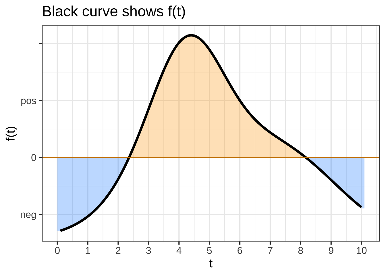
Assume that the “area” of each small box on the graph is the product of 1 Watt \(\times\) 1 second.
askMC(
  "What is $$\\int_1^2 f(t) dt\\ \\text{?}$$ (Choose the closest answer. The units are in Watt-seconds.)",
  -3.2, "-1.4"="Count the boxes in the interval", "0"="Count the boxes in the interval", "2.5"="Count the boxes in the interval", "3.3" = "That's a pretty good count of boxes, but still not the right answer.", 6.1, right_one = -3.2,
  random_answer_order = FALSE
)
What is $$$\int_1^2 f(t) dt\ \text{?}$$$ (Choose the closest answer. The units are in Watt-seconds.)
(x ) -3.2
( ) -1.4
( ) 0
( ) 2.5
( ) 3.3
( ) 6.1
[[Good.]]
\[\text{Let}\ \ A = \int_1^3 f(x) dx\ \ \ \text{and}\ \ \ B = \int_2^4 f(x) dx\]
askMC(
  "Which is bigger, A or B?",
  "A", "B", "They are the same size", right_one = "B",
  random_answer_order = FALSE
)
Which is bigger, A or B? ( ) A (x ) B ( ) They are the same size [[Correct.]]
\[\text{Let}\ \ A = \int_3^1 f(t) dt\ \ \ \text{and}\ \ \ B = \int_4^2 f(t) dt\]
askMC(
  "Which is bigger, A or B?",
  "A", "B", "They are the same size", right_one = "A",
  random_answer_order = FALSE
)
Which is bigger, A or B? (x ) A ( ) B ( ) They are the same size [[Right!]]
Consider the function \[g(x) \equiv \int_4^x f(t) dt\] for the next three questions
askMC(
  "Which is bigger, $g(8)$ or $g(9)$?",
  "+$g(8)$+", "$g(9)$"="the interval from 8 to 9 decreases the total size", "They are the same size",
  "Trick question! There can be no such function $g(x)$ since $f()$ is a function of $t$" = "Try plugging in $x=8$ on the right side of the definition and see if it makes sense."
)
Which is bigger, $$g(8)$$ or $$g(9)$$? (x ) $$g(8)$$ ( ) $$g(9)$$ ( ) They are the same size ( ) Trick question! There can be no such function $$g(x)$$ since $$f()$$ is a function of $$t$$ [[Right!]]
askMC(
  "Is $g(2.5)$ positive or negative?",
  "positive" = "The function being integrated, $f(t)$, is positive over the interval $2.5 \\leq t \\leq 4$. Since the lower limit $t=4$ is larger than the upper limit $t=2.5$, the $\\int_4^{2.5} f(t)dt$ is negative.", "zero", "+negative+"
)
Is $$g(2.5)$$ positive or negative? ( ) positive ( ) zero (x ) negative [[Nice!]]
askMC(
  "At what value of $x$ is $g(x) = 0$?",
  "2"="There is still area under the curve for this interval", "3"="There is still area under the curve for this interval", "4" = "When the two limits of integration are the same, the definite integral is *always* zero.", "5"="There is still area under the curve for this interval", "6"="There is still area under the curve for this interval", "7"="There is still area under the curve for this interval", "8"="There is still area under the curve for this interval", right_one = 4,
  random_answer_order = FALSE
)
At what value of $$x$$ is $$g(x) = 0$$? ( ) 2 ( ) 3 (x ) 4 ( ) 5 ( ) 6 ( ) 7 ( ) 8 [[When the two limits of integration are the same, the definite integral is *always* zero.]]
\[\text{Let}\ \ h(x) \equiv \int_0^x f(t) dt\]
askMC(
  "At what value of $x$ is $h(x) \\approx 0$?",
  "1"="consider when positive and negative areas are equal in magnitude.", "2"="consider when positive and negative areas are equal in magnitude.", "3"="consider when positive and negative areas are equal in magnitude.", 4, "5"="consider when positive and negative areas are equal in magnitude.", "6"="consider when positive and negative areas are equal in magnitude.", right_one = 4,
  random_answer_order = FALSE
)
At what value of $$x$$ is $$h(x) \approx 0$$? ( ) 1 ( ) 2 ( ) 3 (x ) 4 ( ) 5 ( ) 6 [[Nice!]]
\(\partial_x h(x)\) is a function. When we write \(\partial_x h(3)\) we mean to evaluate that function for an input value of \(x=3\).
askMC(
  "Which is bigger, $\\partial_x h(3)$ or $\\partial_x h(4)$?",
  "$\\partial_x h(3)$"="remember $f(t) is essentially the derivative of $h(x)$ with respect to x.","+$\\partial_x h(4)$+", "Can't tell."
)
Which is bigger, $$\partial_x h(3)$$ or $$\partial_x h(4)$$? ( ) $$\partial_x h(3)$$ (x ) $$\partial_x h(4)$$ ( ) Can't tell. [[Nice!]]
\[\text{Let}\ \ y(x) \equiv \int_4^x f(t) dt\]
Here are four different graphs.
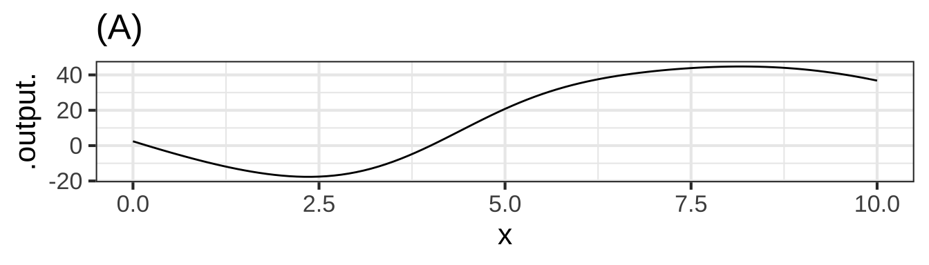
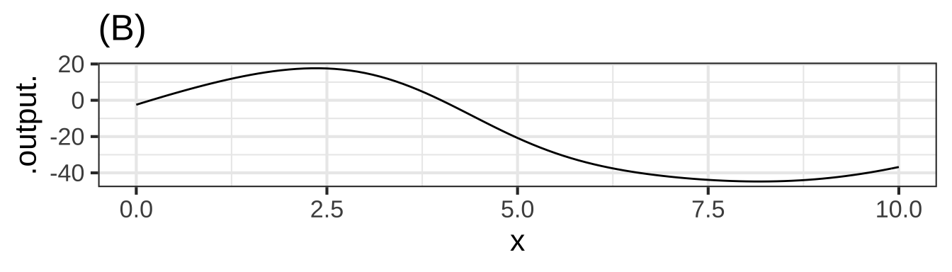
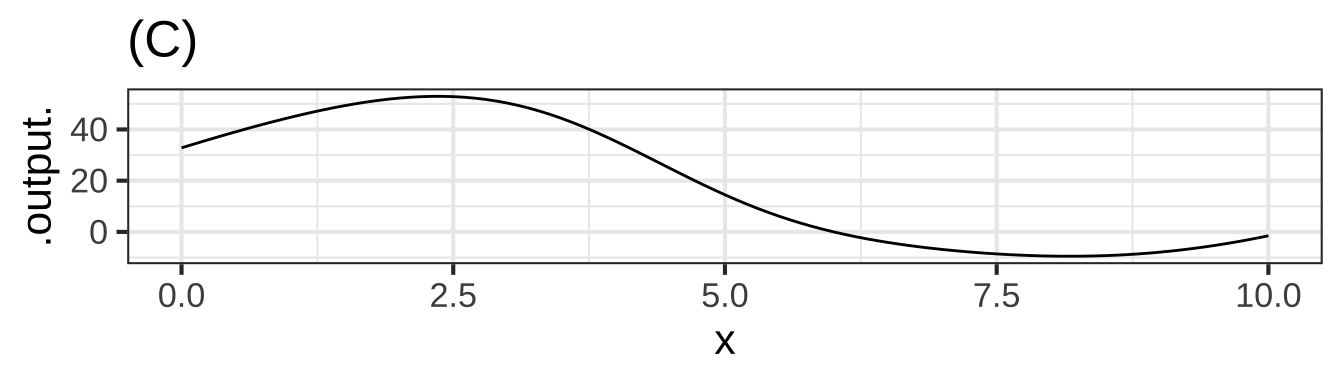
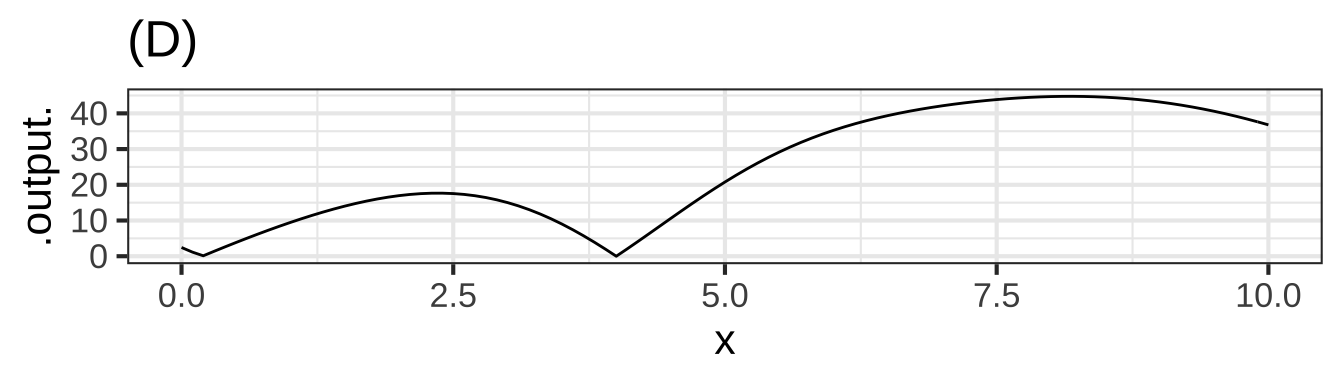
askMC(
  "Which of the graphs shows $y(x)$?",
  "A", "B"="Should it increase or decrease after the point crosses the x-axis?", "C"="Should it increase or decrease after the point crosses the x-axis?", "D"="When should the graph equal 0?", right_one = "A",
  random_answer_order = FALSE
)
Which of the graphs shows $$y(x)$$? (x ) A ( ) B ( ) C ( ) D [[Excellent!]]
Exercise 30.08: 9W6VB
Using the Euler method find \(\int f(t) dt\) over the interval \(t_0=0\) to \(t_{end}=1\). The \(t\) quantity is in steps of \(h=0.01\).
| \(t\) | \(\partial_t f(t)\) | \(\int f(t) dt\) |
|---|---|---|
| 0 | 0.399 | 0.5 |
| 0.01 | 0.242 | |
| 0.02 | 0.054 |
Exercise 30.10: 3IU9R
Consider this sequence: 4, 5, 3, 1, 2
What is the sum?


( )  14
(x )  15
( )  16
( )  17

[[Yes, we know you can add. We just wanted you to keep in mind what the sum is for the next question, which is just about as easy.]]
What is the cumulative sum?


(x )  The sequence 4, 9, 12, 13, 15
( )  The sequence 2, 3, 6, 11, 15
( )  The sequence 0, 4, 9, 13, 15

[[Right!]]
Which entry in the cumulative sum matches the sum?


( )  The first
(x )  The last
( )  None of them
( )  All of them

[[Good.]]
Exercise 30.12: ljCxcH
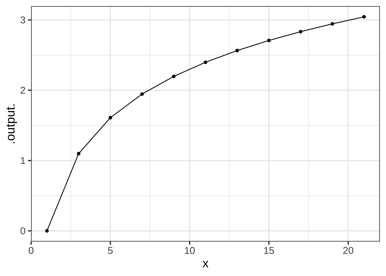
The result of applying the Euler method to a function is also another function, but it comes in the form of a vector of numbers all ready to be displayed graphically. So keep in mind the the function produced by Euler will be known only over a specified domain, just as the graph of a function covers only the specified domain. For instance, here is the graph of the natural logarithm function over the domain \(1 \leq x \leq 21\).
The command in the sandbox is a little different than the usual slice_plot(). We’ve added on two things:
An argument
npts=11which says to use 11 discrete values of the input in plotting the graph.A second graphics layer that shows a dot at each input point where
slice_plot()evaluated the function. Behind the seemingly smooth curves thatslice_plot()produces is really a discrete set of points each of which is the output of the function at some numerical input.
In our typical use of slice_plot() we leave out the dots and show only the straight line segments that connect the positions where the dots would be plotted. If the positions are spaced closely enough, your eye will not see the joints between successive straight lines and you will perceive the graph as a smooth curve.
For the graph of the log function over the domain $$1 \leq x \leq 21$$ with `npts=11` (that is, the initial command shown in the sandbox), what is the horizontal spacing between the discrete $$x$$ values?


( )  0.5
( )  1
(x )  2
( )  4
( )  5

[[Excellent!]]
Now take away the npts= argument. This will implicitly set npts to a default value, which is what we have been using for most plots in this course.
What is the default value of `npts` in `slice_plot()`?


( )  25
( )  50
(x )  100
( )  200
( )  500
( )  1000

[[Correct.]]
We could use a much larger value for npts, but there is no reason so long as a smaller value produces a graph faithful to the function being graphed.
Keeping the domain the same, \(1 \leq x \leq 21\), plot out a sinusoid with a period of 0.3 using the default npts: \(g(x) \equiv \sin(2\pi x/0.3)\). The graph, which shows about 67 cycles of the sinusoid, will not look much like a sinusoid. In particular, although the sine function should reach from -1 to 1 over each cycle, the graph does not.
How large should `npts` be in order for each of the 67 cycles in the graph to come close enough to -1 and 1 that you cannot easily see the discrepancy?


( )  125
( )  150
( )  200
( )  400
(x )  800
( )  1600
( )  3200

[[Excellent!]]
Exercise 30.14: rfO0EG
Methods such as Euler are tedious, ideal for the computer. So let’s look at some basic R functions for implementing the Euler Method when we know the function to be anti-differentiated \(f(x)\), the step size \(h\), and the domain \(a \leq x \leq b\). At the heart of the implementation is a function cumsum(), the “cumulative sum.” This does something very simple. The cumulative sum of the sequence 1, 2, 3, 4 is another sequence: 1, 3, 6, 10.
The following code has commands for using cumsum() to approximate the anti-derivative of a function \(f()\) over the domain \(a \leq x \leq b\)
f <- makeFun(sin(2*pi*x/0.3) ~ x) # the function to be anti-differentiated.
a <- 1 # the lower bound.
b <- 2 # the upper bound.
h <- 0.01 # the step size
x_discrete <- seq(a, b, by = h) # all of the discrete x values based on a, b, and h
f_discrete <- f(x_discrete) # all of the values of f(x) when the discrete x values are used as the input
F_discrete <- cumsum(h * f_discrete) # the discrete values of the anti-derivative, F(x)
gf_point(F_discrete ~ x_discrete) %>%
  slice_plot(f(x) ~ x, color = "gray", domain(x=c(a,b)))
Here is a function:
g <- makeFun(exp(-0.2*(x^2))~x)Using a SANDBOX, find and plot the anti-derivative of \(g(x)\) over the domain \(-6 \leq x \leq 6\).
Your task: Describe the shape of \(G(x)\). Your description can be one word from earlier in the book, if you choose it carefully. If your graph looks like a straight line, you did not appropriately change the domain above.ECONOMIST PICTURES
knitr::include_graphics("www/sputnik.png")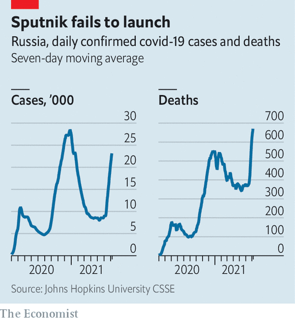
knitr::include_graphics("www/NHS.png")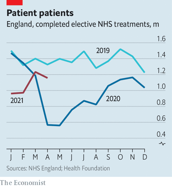
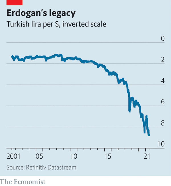
knitr::include_graphics("www/Turkish-lira.png")