Chapter 10 So-called “statistical significance”

In this book we’ve used effect size as the basic measure of how a response variable is related to an explanatory variable. The confidence interval of an effect size tells what range of values are consistent with our data. When that interval includes zero, it’s fair to say that our data do not rule out the possibility that there is no effect at all, that is, that the response and explanatory variables are unrelated.

For historical reasons, its common for researchers to present their results as “statistically significant.” The way a relationship between a respose and explanatory variable(s) can win the certificate of “statistical significance,” is by a process called null hypothesis testing. A null hypothesis test involves calculating a quantity known as the p-value, which is always between 0 and 1. When the p-value is smaller than 0.05 (by convention), the researcher is warranted in using the label “statistically significant.”

First, I’ll handle the question of how the calculation is done. Then, I’ll give some history and recent professional recommendations that the result of the calculation has no meaning. Hopefully, despite the ubiquity of p-values in conventional statistics textbooks and in the research literature, you’ll be able to use more meaningful ways to describe the relationship, if any, between response and explanatory variables.

10.1 Calculating a p-value

When you quantify the relationship between a response and explanatory variable(s), several inferential quantities are generated. In this book, we focus particularly on F and the degrees of flexibility \(df\), from which everything else flows.

The p-value calculation takes F, \(df\) and sample size \(n\) as inputs and produces an output in the form of a probability, that is, a number between 0 and 1. The calculation from first principles is very difficult, so everyone builds on the earlier work of couragious statisticians and mathematicians who have simplifed it into looking up a number in a table, or, more conveniently, asking a computer to look up the number.

For example, in the R computing language, the function \(pf()\) does the calculation. Specifically, the p-value is 1 - pf(F, df, n - df). In many software systems, such as Excel, all of the F, \(df\) and p-value calculations are packaged together in functions that are often called “tests.” There are often many such “tests” provided for different settings like the difference between two means or the slope of a regression line. But the underlying principles are those presented here in a unified way, with \(v_r\), \(v_m\), \(df\), and F.

Since what you do with a p-value is to compare it to 0.05, there is a remarkably simple way to go. instead of making the rule about the size of the p-value, we make it about the size of F. The value of F that corresponds to \(p = 0.05\) is called the “95% critical value” of F. This is often written F\(^\star\). So long as you have \(n\) moderately large, say \(n \gtrapprox 10\), the critical value is 4. That’s it. 4. If \(n \gtrapprox 10\), F=4 is the threshold for declaring a relationship “statistically significant.”

For \(n\) small, it’s no longer adequate to use 4 as the critical value. Instead, for all the situations encountered in an introductory statistics class, you have to look up the critical value in Figure 1.

Sample size \(n\)	large	10	9	8	7	6	5	4	3
F\(^\star\)	4	5	5.3	5.6	6	7	8	10	19

**Figure 1: Critical values for F depend on the sample size \(n\), especially for small \(n\). These critical values are for \(df=1\).

Do remember that the formula for F includes \(n\). One way to get a large F is to use data with large \(n\). So don’t mis-interpret the table as saying “10 points is enough.” It’s just that F\(^\star\) doesn’t much depend on \(n\) when \(n \gtrapprox 10\).

Figure 1 is for \(df = 1\), which is the situation in most of the settings used in introductory statistics. For larger \(df\), the critical values of F are similar except for models where \(df \approx n\). See Figure 3, below.

10.2 History and criticism

In the 1880s a way of quantifying the relationship between two numerical variables was invented. It was called the correlation coefficient and it continues to be used to this day. Probably it should not be so widely used today as it is, because we now have effect sizes to work with and because of the challenges to interpreting the correlation coefficient, as you’ll see.

The correlation coefficient from the 1880s is closely related to the \(R^2\) statistic introduced in Chapter 6. Specifically, the size of the correlation coefficient is \(r = \sqrt{R^2} = R\). Recall that \(R^2\) is the ratio of the variance of model values to the variance of the response variable:

\[R^2 \equiv v_m / v_r.\]

Recall as well that each of \(v_m\) and \(v_r\) are an average of square differences, and, of course, a square of a real number cannot be less than zero. Consequently, \(R^2\) cannot be negative.

If \(R^2\) is exactly zero, it’s reasonable to conclude that the explanatory variable(s) cannot account for the response variable. Seen another way, if \(R^2\) is zero then \(v_m\) must also be zero. For \(v_m\) to be zero, all of the model values must be exactly the same, so the effect size must also be zero.

What happens if – to do a thought experiment – the response variable is completely unrelated to the explanatory variable? You might be anticipating that \(R^2\) will be zero. In practice, however, it’s not. This comes about because there are almost always associations happening purely at random that, when quantified, produce \(R^2 > 0\). So, in deciding whether the data indicate a relationship between the response and explanatory variable(s), we need to decide what value of \(R^2\) is so close to zero as to be a sign that the response and explanatory variable(s) are related.

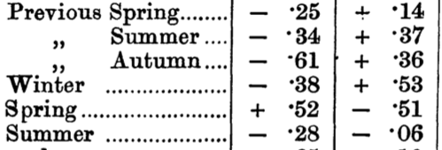
This question was asked, and answered, early in the 1900s. In one specific case, it was asked by a man named Dr Shaw at the January 15, 1907 meeting of the Royal Statistical Society in the UK. The context was a discussion of a paper by Reginald Hooker who had studied the correlation between weather and crops. In Table 1 of his paper, part of which is reproduced in Figure 1, Hooker presented the correlation between amount of wheat harvested and the amount of rain accumulated over the previous seasons. He also looked at the correlation of wheat harvest and temperature – that’s the second numerical column in Figure 2.

Now to quote from the recollections published in 1908 by William Seely Gossett, writing anonymously as “Student”:

Dr Shaw made an enquiry as to the significance of correlation coefficients derived fronm small numbers of cases.

The small number here is 21: Hooker had worked with 21 years of crop and weather data. The plain meaning of “significance of” here is “the meaning carried by.” A modern person might have asked, “Some of those correlations are pretty small. And you don’t have much data. Do such small correlations mean anything?” To continue …

His question was answered by Messrs Yule and Hooker and Professor Edgeworth, all of whom considered that Mr Hooker was probably safe in taking .50 as his limit of significance for a sarnple of 21.

In plainer language: don’t take as meaningful any correlation coefficient less than 0.50.

They did not, however, answer Dr Shaw’s question in any more general way. Now Mr Hooker is not the only statistician who is forced to work with very small samples, and until Dr Shaw’s question has been properly answered the results of such investigations lack the criterion which would enable us to make full use of them. The present paper, which is an account of some sampling experimiients, has two objects: (1) to throw some light by empirical methods on the problem itself, (2) to endeavour to interest mathematicians who have both time and ability to solve it.

A general solution was found, in part by Student but also by others such as Ronald Fisher. Key to setting up the solution was to define “significance” in mathematical terms. The setup was logically ingenious and a little hard to follow. It goes like this:

Suppose we have two variables that have been generated entirely at random and independently of one another. We can calculate the correlation coefficient between them. The correlation coefficient will also be a random number, presumably near zero. If we perform the experiment many times and collect the set of random correlation coefficients produced, we will have an idea of what is the size of commonly encountered coefficients, and how big a correlation coefficient should be so that we can sensibly regard it as being unlikely to arise from random, independent variables.

Doing the random-and-independent-variable simulation for the \(n = 21\) situation of Hooker’s paper, indicates that a correlation coefficient at or above 0.50 will result about 1% of the time. That’s a small probability. So, as Messrs Yule, Hooker, and Edgeworth said, it seems “pretty safe” – 99%? – to conclude that \(r = 0.50\) with \(n=21\) means that there is an association between the two variables.

Actually, the simulation only tells us about a hypothetical world – called the Null Hypothesis – in which variables are random and independent. The simulation doesn’t have anything to say about a world in which variables are related to one another. It’s legitimate to say that observing something that’s very unlikely – 1% chance of \(r \ge 0.5\) – suggests that the data didn’t come from that world. But suppose data came from another hypothetical world – called the Alternative Hypothesis – where variables are related to one another. Such a world might easily generate a value \(r < 0.5\). So seeing large r entitles us to “reject the null hypothesis,” but seeing small r doesn’t tell us about the alternative hypothesis. Small r just means that we can’t reject the null hypothesis. The formal language is “fail to reject the null hypothesis.”

The probability that comes from the null hypothesis simulation has a name: the p-value.

In 1925, Ronald Fisher suggested using a probability of 5% instead of 1% in lab work. This guideline was intended to help lab workers avoid making unwarranted claims that an experiment is showing a positive result. If the p-value is \(p > 0.05\), you have nothing to say about your experiment, you fail to reject the null hypothesis.

Over the years, this got turned around. When \(p < 0.05\) (by convention), you’re entitled to “reject the null hypothesis.” In order to publish a scientific report, researchers were obliged to have enough data to reject the null. This is a way of saying that some non-null claim is warranted. But which ones? Certainly the point is to show that there is some substantial relationship between the response and explanatory variable(s), a relationship that means something in the real world. Rejecting the null is not, on its own, a sign that the relationship is substantial and meaningful.

Further confusing things was that little word used by Dr Shaw in 1907: significance. An equivalence developed between “reject the null” and “significance.” Claims that had a low p-value came to be described as “statistically significant.” In everyday speech, “significant” means substantial or meaningful or important. This is not the meaning of “statistically significant.” The importance or meaning of an association between a response and explanatory variables can be assessed by looking at the effect size, and checking whether the effect size is large enough to have practical meaning in the world. But even tiny effect sizes, without any practical implications, can generate small p-values. You just have to have enough data. With the phrase “statistically significant” attached to findings, people could publish their work even if there was no practical meaning.

It’s worse than this. Even when variables are unrelated, the p-value will be smaller than 0.05 on five percent of occasions. When Fisher was writing in 1925, there weren’t many researchers and each lab experiment required a lot of work. And, in any event, “rejecting the null” was just an internal check on what lab work is worth following up and replicating. But today there are millions of researchers. And each researcher can easily look at dozens of variables. So, even if every researcher was working with unrelated variables, statistical significance will be found millions of times: enough to saturate the literature and effectively hide genuine findings with practical significance.

After decades of researchers mis-using p-values, in 2019 the American Statistical Association, a leading professional organization world-wide, issued a statement worth quoting in length:

It is time to stop using the term ’statistically significant" entirely. Nor should variants such as “significantly different,” “p < 0.05,” and “nonsignificant” survive, whether expressed in words, by asterisks in a table, or in some other way.

Regardless of whether it was ever useful, a declaration of “statistical significance” has today become meaningless. Made broadly known by Fisher’s use of the phrase (1925), Edgeworth’s (1885) original intention for statistical significance was simply as a tool to indicate when a result warrants further scrutiny. But that idea has been irretrievably lost. Statistical significance was never meant to imply scientific importance, and the confusion of the two was decried soon after its widespread use (Boring 1919). Yet a full century later the confusion persists.

And so the tool has become the tyrant. The problem is not simply use of the word “significant,” although the statistical and ordinary language meanings of the word are indeed now hopelessly confused (Ghose 2013); the term should be avoided for that reason alone. The problem is a larger one, however: using bright-line rules for justifying scientific claims or conclusions can lead to erroneous beliefs and poor decision making (ASA statement, Principle 3). A label of statistical significance adds nothing to what is already conveyed by the value of p; in fact, this dichotomization of p-values makes matters worse.

For example, no p-value can reveal the plausibility, presence, truth, or importance of an association or effect. Therefore, a label of statistical significance does not mean or imply that an association or effect is highly probable, real, true, or important. Nor does a label of statistical nonsignificance lead to the association or effect being improbable, absent, false, or unimportant. Yet the dichotomization into “significant” and “not significant” is taken as an imprimatur of authority on these characteristics. In a world without bright lines, on the other hand, it becomes untenable to assert dramatic differences in interpretation from inconsequential differences in estimates. As Gelman and Stern (2006) famously observed, the difference between “significant” and “not significant” is not itself statistically significant.

Furthermore, this false split into “worthy” and “unworthy” results leads to the selective reporting and publishing of results based on their statistical significance—the so-called “file drawer problem” (Rosenthal 1979). And the dichotomized reporting problem extends beyond just publication, notes Amrhein, Trafimow, and Greenland (2019): when authors use p-value thresholds to select which findings to discuss in their papers, “their conclusions and what is reported in subsequent news and reviews will be biased…Such selective attention based on study outcomes will therefore not only distort the literature but will slant published descriptions of study results—biasing the summary descriptions reported to practicing professionals and the general public.” For the integrity of scientific publishing and research dissemination, therefore, whether a p-value passes any arbitrary threshold should not be considered at all when deciding which results to present or highlight.

10.3 Appendix: When \(df \geq 2\)

For models with multiple explanatory variables or categorical variables with more than two levels, the critical values of F differ substantially from the \(df = 1\) case only for very small \(n\).

Sample size \(n\)	large	10	9	8	7	6	5	4	3
\(df = 1\)	4	5	5.3	5.6	6	7	8	10	19
\(df = 2\)	3	4.5	4.7	5.1	5.7	7	9.5	19	200
\(df = 3\)	2.7	4.3	4.8	5.4	6.6	9.3	19	216	NA
\(df = 4\)	2.5	4.5	5.2	6.4	9.1	19	225	NA	NA

Figure 3: Critical values for F for small \(n\) and a few different values of \(df\).