Chapter 12 Comparing models

Up to now, we have looked at models individually. It’s time now to examine models in pairs. Such a perspective gives insight into constructing models, for example by including a new explanatory variable in addition to the old ones, or increasing the curvature used in a model function.

The basic strategy is simple. Start with an existing model, which we might call $\hbox{mod}_1$. Then extend or elaborate $\hbox{mod}_1$ in some way, perhaps by including a new explanatory variable to produce $\hbox{mod}_2$. We can then examine the increase in the variance of the model values from what it was under $\hbox{mod}_1$ to what it will be under $\hbox{mod}_2$.

Since we are working with two models, it’s helpful to modify the notation a bit. Before, we had $\hbox{v}_r$ and $\hbox{v}_m$, the variance of the response variable and of the model values respectively. We also had R², which is simply $\hbox{v}_m$ divided by $\hbox{v}_r$. We’ll keep $\hbox{v}_r$ as standing for the variance of the response variable but write $\hbox{v}_1$ and $\hbox{v}_2$ as the variance of the model values from $\hbox{mod}_1$ and $\hbox{mod}_2$ respectively.

Likewise, it’s useful to construct the R-squared ratios for the two models, which we’ll denote $\hbox{R}^2_1$ and $\hbox{R}^2_2$, and which are simply $\hbox{v}_1 / \hbox{v}_r$ and $\hbox{v}_2 / \hbox{v}_r$ respectively.

12.1 Complexity and cost

A central question when considering an extending $\hbox{mod}_1$ into $\hbox{mod}_2$ is whether the resulting increase in variances, $\Delta \mbox{v} = \hbox{v}_2 - \hbox{v}_1$ is large enough to justify concluding that extending $\hbox{mod}_1$ to $\hbox{mod}_2$ is worth the cost.

The “cost?” What cost? Computing the new model $\hbox{mod}_2$ and its model values is, with a computer, trivial and costs nothing. Rather, the cost of concern is the added complexity of $\hbox{mod}_2$ compared to $\hbox{mod}_1$.

There is a tradition in science of assuming that, all other things being equal, simpler models are better than more complicated models. Sometimes this tradition is expressed as the “law of parsimony,” as if it were a physical principle (which it is not, until you get very deep into things as in quantum electrodynamics). Sometimes it is given the name “Occams’s Razor” in honor of William of Ockham (c. 1287–1347). Occam’s Latin statement is

“Numquam ponenda est pluralitas sine necessitate.”

The English translation is scarcely better: “Plurality must never be posited without necessity.” A somewhat earlier formulation might be clearer:

“It is superfluous to suppose that what can be accounted for by a few principles has been produced by many.” – Thomas Aquinas (1225–1274)

It’s deeply ironic that opinions from the 13th century be quoted as support for scientific principles. At the start of the 20th century, however, some relevant mathematics started to emerge, the mathematics of random walks. This new mathematics provided insight into how complexity of a model might be measured and a criterion for judging whether adding complexity is worthwhile.

We’ll put the mathematical theory in a framework that we’ve already developed in earlier chapters. The ingredients are

n, the number of rows in the data used to construct the model
$^\circ\!{\cal{F}}_1$ and $^\circ\!{\cal{F}}_0$ the degrees of flexibility of $\hbox{mod}_2$ and $\hbox{mod}_1$ respectively.
$\hbox{R}^2_2$ and $\hbox{R}^2_1$

Here are some relevant facts resulting from the mathematical theory of random walks.

Fact 1: If $\hbox{mod}_2$ is an extension of $\hbox{mod}_1$ (for instance, one created by including an additional explanatory variable) then $\hbox{v}_2 \geq \hbox{v}_1$.

Justification: Reach back to Chapter 5 where we considered the process of creating a model function. Recall that the “best” model function is one that comes as close to the response variable as possible, given the selected set of explanatory variables. In extending $\hbox{mod}_1$, we are giving the process an additional variable to work with. Likely, there will be some way to use that additional variable so that $\hbox{mod}_2$ gets even closer to the response variable than $\hbox{mod}_1$. But simply by ignoring the additional variable, $\hbox{mod}_2$ can at least as close as $\hbox{mod}_2$.
Fact 2: Suppose that all of the explanatory variables are unrelated to the response variable, for instance, they have been created at random. Then a model constructed with n-1 degrees of flexibility will have $\hbox{v}_m = \hbox{v}_r$. What’s more, a model with $p < n-1$ degrees of freedom will, on average, have $\hbox{v}_m \approx \frac{p}{n-1} \hbox{v}_r$. Another way of stating this is that \[R^2 = \frac{\hbox{v}_m}{\hbox{v}_r} \approx \frac{p}{n-1}\]

In support of Fact 2, we’ll do some simulations. In each trial, we’ll generate a small data set with $n=11$. The response variable will come from a random number generator. Similarly we’ll make up p=5 explanatory variables, each of which is also from a random number generator. Then we’ll calculate R² from each model and look at the distribution. According to the principle, on average

$R^2 = \frac{p}{n-1} = \frac{5}{10}$.

We’ll do the simulation using R software and the mosaic package. I provide the code so that anyone who wants to carry out their own simulation can do so. We’ll do 1000 trials.

library(mosaic)

Trials <-  do(1000) * (
  data.frame(y  = rnorm(n = 11)) %>%
    lm(y ~ rand(5), data = .) %>%
    rsquared()
)
mean( ~ result,  data = Trials)

## [1] 0.498377

You can repeat the simulation with any n and p that you like to confirm that, on average, $R^2 \approx \frac{p}{n-1}$.

## Warning: `data_frame()` is deprecated, use `tibble()`.
## This warning is displayed once per session.

12.2 Why F?

We can use Fact 2 to explain why it makes sense for the F-statistic to be defined the way it is. Consider a graph of the average R² versus $^\circ\!{\cal{F}}$ when all the explanatory variables are made with a random number generator

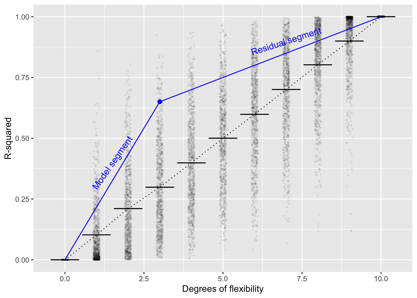
Figure 12.1: (ref:RandomR-cap)

In Figure 12.1, the blue point falls at R²=0.65 and $^\circ\!{\cal{F}} = 3$. Referring to the individual random trials with $^\circ\!{\cal{F}} = 3$ (the black dots), you can see that a very small percentage have R² > 0.65. This alone would cause one to doubt that the explanatory variables used in making the blue dot were purely random. In fact, a p-value for the blue dot could be calculated simply by counting the proportion of black dots that have R-squared larger than the blue dot (for $^\circ\!{\cal{F}} = 3$).

This book is about classical inference, so the use of simulation, a computer-era technique, is out of place. Classical inference resorts to a different observation. In Figure 12.1, there are two blue segments. One connects the origin to the blue dot, the other connects the blue dot to the upper-right corner of the plot. We’ll call the left-most segment the “model segment,” since it reflects Clearly the slope of segment one is larger than the slope of segment two. This will happen whenever the blue dot is above the vertical range of the random trials. But for the random trials, on average, the two slopes would be about the same. So, under the Null Hypothesis that the explanatory variables are unrelated to the response variable, the ratio of slopes will be about 1.

Fisher suggested using the ratio of slopes in the R² versus $^\circ\!{\cal{F}} = 3$ graph as a test statistic. Given a blue dot with its R² and $^\circ\!{\cal{F}} = 3$, the slope of segment one is $\mbox{R}^2_1 / ^\circ\!{\cal{F}}$. Similarly, the slope of segment two is $(1 - \mbox{R}^2_2) / (n - (^\circ\!{\cal{F}} +1))$. The ratio of slope one to slope two is F.

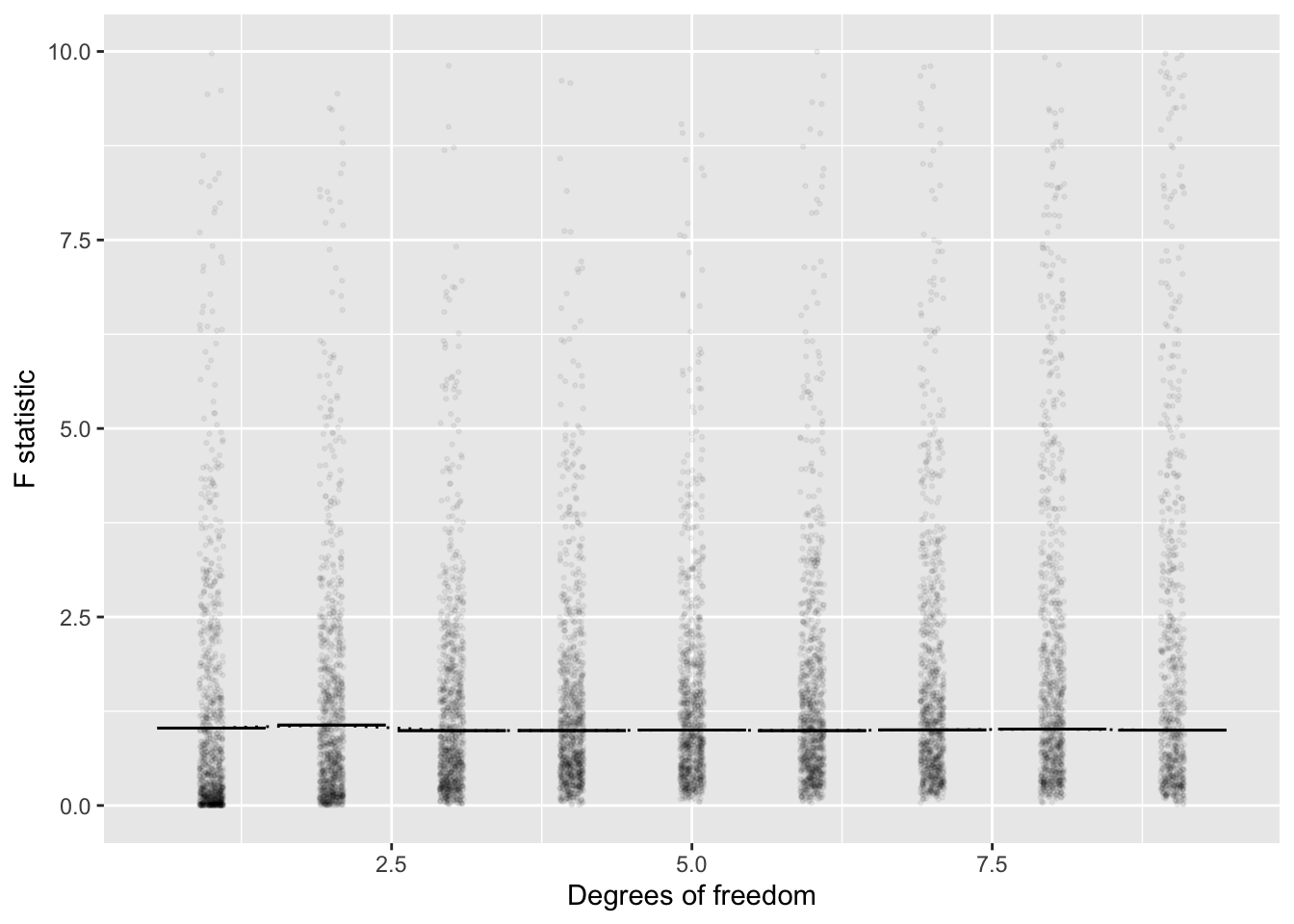
$Figure 12.2. Translating the $R^2$ and $^\circ\!{\cal{F}}$ values from Figure 12.1 into the corresponding F value shows a much simpler version. On average, the F values from the random simulation are about $F=1$ regardless of $^\circ\!{\cal{F}}$. Similarly, almost all the random trials produce $F < 4$. Fisher deduced these facts using algebra and calculus with the mathematics of random walks, a remarkable achievement. Today, it takes only a moderate amount of computer-programming skill to confirm them.$

Figure 12.2: Figure 12.2. Translating the $R^2$ and $^\circ\!{\cal{F}}$ values from Figure 12.1 into the corresponding F value shows a much simpler version. On average, the F values from the random simulation are about $F=1$ regardless of $^\circ\!{\cal{F}}$. Similarly, almost all the random trials produce $F < 4$. Fisher deduced these facts using algebra and calculus with the mathematics of random walks, a remarkable achievement. Today, it takes only a moderate amount of computer-programming skill to confirm them.

12.3 Analysis of variance

The word “analysis” refers to the process of breaking something down into its constituent components. (The antonym is “synthesis,” the process of bringinging components together to form a whole.)

The phrase “analysis of variance” concisely describes the strategy for examining a model that consists of components. For example, we’ve described $\hbox{mod}_2$ as being an extension of $\hbox{mod}_1$ – mod_2 consists of $\hbox{mod}_1$ plus some additional component.

In undertaking analysis of variance, the quantity that is being broken down is the variance r of the response variable. When working with a single model, the variance is broken down into two components:

m, the variance accounted for by the model
what’s left over, the residual variance, which is simply r - m.

In the previous section, I’ve chosen to report not the variance itself, but the proportion of the variance of the response variable:

$R^2 = \hbox{v}_m / \hbox{v}_r$, the proportion accounted for by the model
$1 - R^2 = (\hbox{v}_r - \hbox{v}_m) / \hbox{v}_r$, the residual proportion of the variance.

The idea of analysis of variance can be extended to the situation of a model $\hbox{mod}_2$ which has been built as an extension to a model $\hbox{mod}_1$. The situation is sketched in Figure 12.3. First, calculate $\hbox{R}^2_1$, the proportion of the variance accounted for by $\hbox{mod}_1$. Second, calculate $\hbox{R}^2_2$, the proportion of the variance captured by $\hbox{mod}_2$. In Figure 12.3, $\hbox{R}^2_1$ is the left-most blue dot, while $\hbox{R}^2_2$ is the other blue dot.

The two blue dots divide the domain of the graph into three components: the model-one segment, the model-two segment, and the residual segment.

To address the question of whether $\hbox{mod}_2$ meaningfully extends $\hbox{mod}_1$, we compare the slope of the model-two segment to that of the residual segment. This ratio of slopes, which we can call $\Delta \hbox{F}$, is the test statistic. If $Delta\hbox{F} \gtrapprox 4$, it’s fair to conclude that the extension to $\hbox{mod}_1$ is discernably different from an extension that would have been concocted from random explanatory variables unrelated to the response variable.

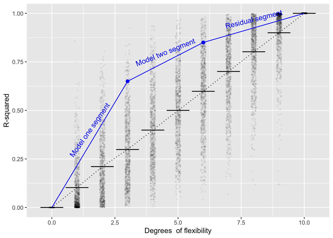
$Figure 12.3: looking at how the extensions to $\hbox{mod}_1$ contained in $\hbox{mod}_2$ increase $\mbox{R}^2_2$ compared to $\mbox{R}^2_1$$

Figure 12.3: Figure 12.3: looking at how the extensions to $\hbox{mod}_1$ contained in $\hbox{mod}_2$ increase $\mbox{R}^2_2$ compared to $\mbox{R}^2_1$

As a formula, the ratio of the slopes of the model-two segment to the model-one segment is:

\[\Delta \mbox{F} = \frac{n - (^\circ\!{\cal F}_{2} + 1)}{^\circ\!{\cal F}_{2} - ^\circ\!\!{\cal F}_{1}} \cdot \frac{\hbox{R}^2_{2} - \hbox{R}^2_{1}}{1 - \hbox{R}^2_{2}}\]

12.4 Analysis of co-variance

It sometimes happens that $\hbox{mod}_1$ contains all the explanatory variables of direct interest and the point of building $\hbox{mod}_2$ is to include those covariates which ought to be taken into consideration but are not of direct interest. In this situation, the ratio of interest is the slope of the model-one segment to the slope of the residual segment. This is called “analysis of co-variance.”

I like to describe the purpose of including the covariates in $\hbox{mod}2$ as “eating variance.” That is, the covariates can reduce the slope of the residual segment, making it easier for the model-one segment to look steep by comparison.