Chapter 6 Degrees of flexibility

\(\newcommand{\flex}[]{^\circ\!{\cal{F}}}\)

Chapter 4 introduced four different settings for models. (For easy reference, Figure 6.1 redraws the examples from Chapter 4.) Remember that the word “settings” is not about the situation that produced the data or the names of the variables being displayed. “Settings” refers to the kind of response variable and explanatory variable – categorical or numerical – begin used in the model.

This chapter introduces some important new settings:

• Settings with more than one explanatory variable
• Settings where a categorical explanatory variable has more than two levels.
• Settings where the straight-line functions seen in Figure 1(b) and 1(d) are replaced with more flexible curves.

It’s far from obvious, but these new kinds of settings are all the same kind of thing mathematically, so statistical inference can handle them in the same way. The central concept that links the new settings is called the degrees of flexibility. For brevity, I’ll use symbols rather than the whole phrase “degrees of flexibility,” a degree sign followed by a flexible-looking F, that is: \(\flex\).

6.1 One degree of flexibility

Each of the models presented in Chapter 4 has a single degree of flexibility, that is, \(\flex = 1\). You can think about degrees of flexibility as how many numbers are required to specify the model completely. For instance, the straight-line models in Figure 6.1(b) and 6.1(d) each can be specified by a slope and an intercept. The models in Figure 6.1(a) and 6.1(b) can be specified by two numbers: the value of the model for the left group and the value for the right group.

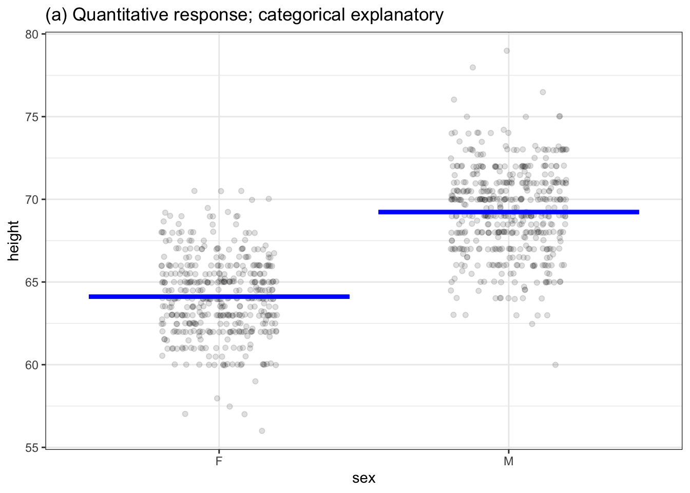
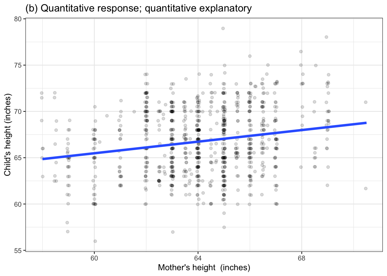
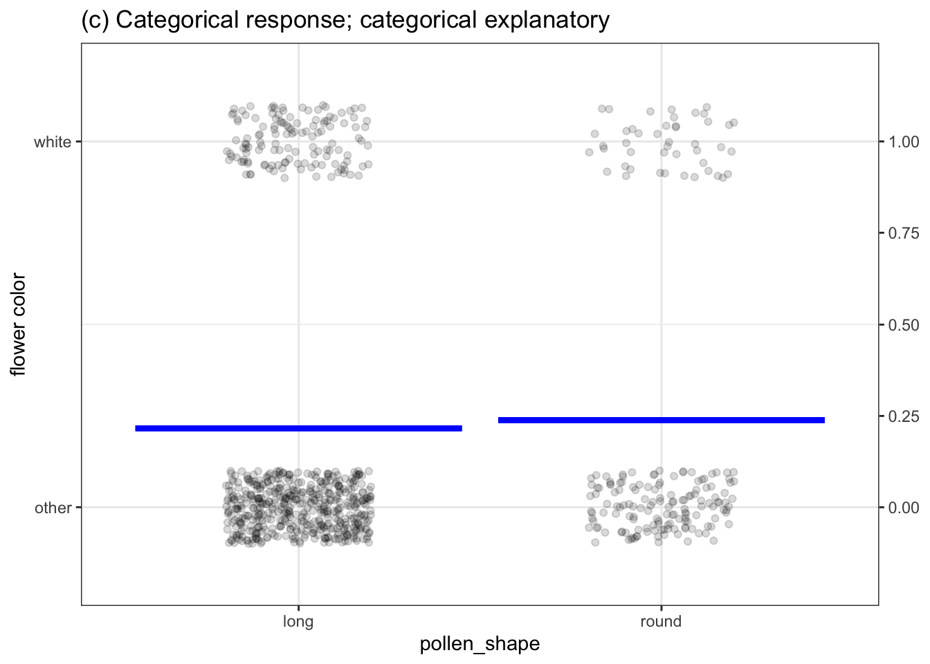
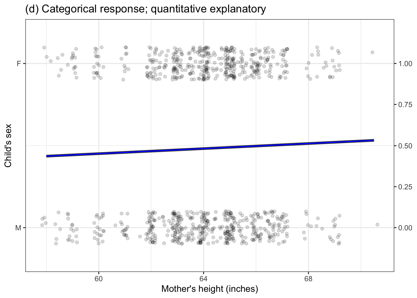
Figure 6.1: Four settings for modeling presented in Chapter 4. All of these have one degree of flexibility, written \(\flex=1\).

In talking about descriptions of models, rather than using the word number, we use coefficient. This is no big deal, but when you see the word coefficient you’ll have a distinct hint that we are talking about the shape of a model. And we’ll be able to say things like “the number of coefficients” to refer to how many coefficients are needed to specify the model.

The degree of flexibility of a model is defined to be the number of coefficients needed to completely specify the model minus one. You might wonder, “Why subtract one from the number of coefficients?” Just a convention. You’ll see some justification for it in Chapter 8, Simple means and proportions, where we will work with models with zero degrees of freedom, which is to say, one coefficient.

6.2 Multiple degrees of flexibility

Let’s look at some examples of models where there is more than one degree of freedom. To start, Figure 2 shows a model with two degrees of freedom: \(\flex = 2\).

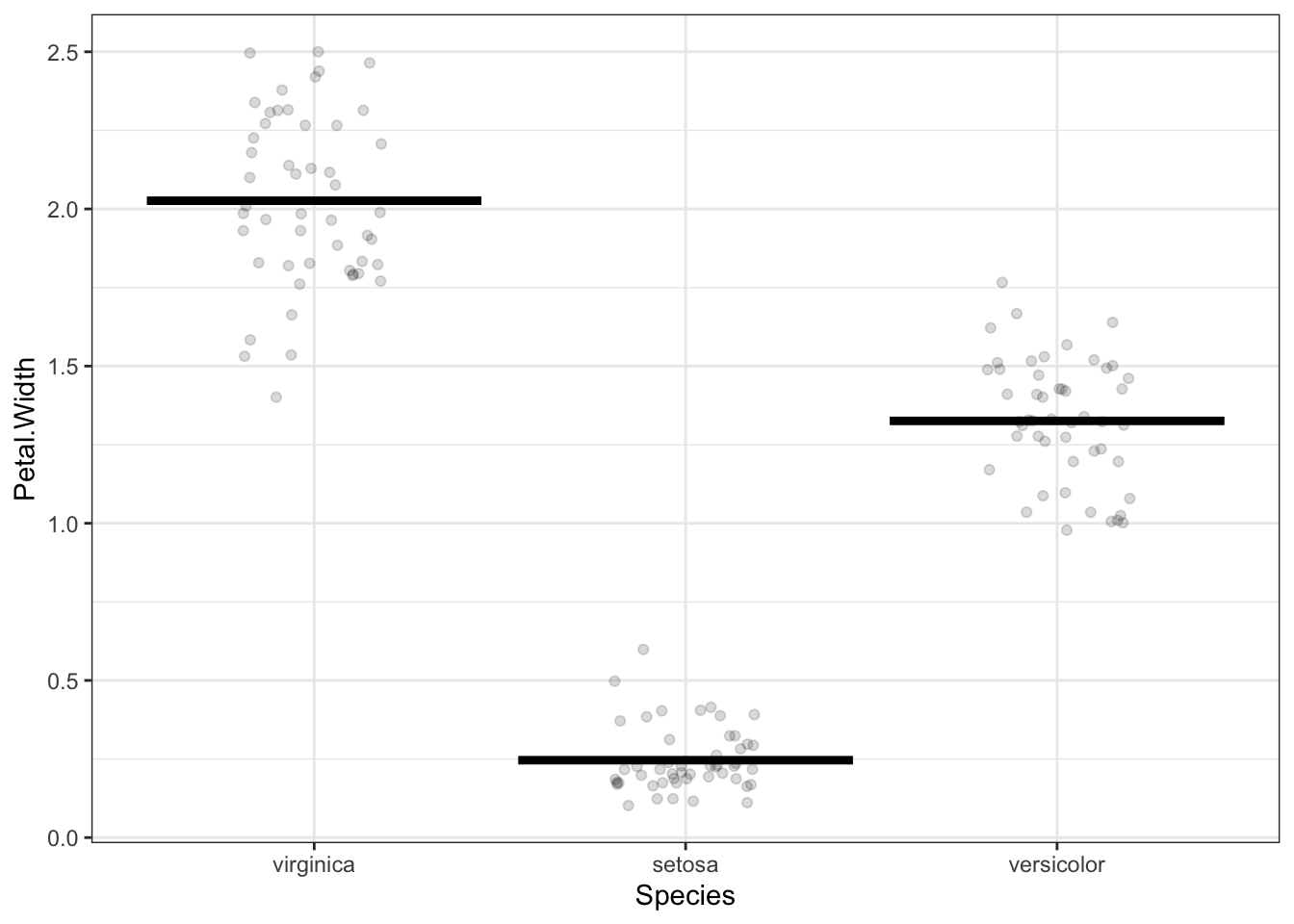
Three coefficients are needed to specify the model values for a model where the 3-level categorical variable Species is the explanatory variable.

The data in Figure 2 are from a classic study involving the differences and similarities among three species of iris plants. The response variable is the flower petal width (quantitative) and the explanatory variable is the species of the plant (categorical). A complete description of the model would involve three coefficients, one for each of the species of iris. Three coefficients corresponds to \(\flex = 2\).

If the explanatory variable had four levels, there would be \(\flex=3\), and so on.

There’s just a single explanatory variable in Figure 2 (albeit one with three categorical levels). Many models have more than one explanatory variable. Figure 3 shows an example, where the response variable is height and bother mother’s height and child’s sex are being used as explanatory variables.

The model in Figure 3 consists of two straight lines. Each line is specified by a slope and an intercept, meaning that four coefficients are needed. Thus, \(\flex=3\).

You may notice that the two lines in Figure 3 have slightly different slopes. Often, modelers try to economize with degrees of flexibility by using the same slope for each line. This would reduce the degrees of freedom to \(\flex = 2\). (The decision of whether to use a common slope or two potentially different slopes is often made using the tools of statistical inference, but we are getting ahead of the story.)

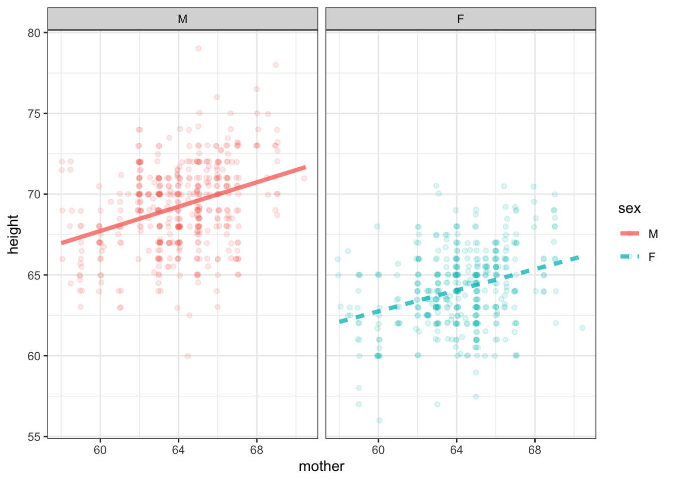
Figure 3: A model of height with two explanatory variables: the mother’s height and the child’s sex. Each explanatory variable added to a model makes it possible for the model more faithfully to reproduce the response variable.

6.3 Covariates

This is a good time to introduce an important concept in statistical modeling. It doesn’t have directly to do with the mechanics of statistical inference, but it is critical to interpreting models with multiple explanatory variables.

Often, there is particular interest in the relationship between two variables. Galton’s interest was in the relationship between the parents’ height and the child’s height. There may be other factors involved in the system – with height a major factor is the sex of the child, but there could be others such as nutrition, health, etc.

Common sense suggests holding these other factors constant so that you can look specifically at the single explanatory variable of particular interest. In the 1880s, Galton did this by considering only the heights of boys rather than the heights of all children. Within a few years of Galton’s work, statisticians had developed techniques to build models with multiple explanatory variables, like Figure 3, which broadened the notion of “holding other factors constant” to include accounting for those factors in a model.

The factors that the modeler wants to hold constant are called covariates. Really this is just a name for an explanatory variable which is not of direct interest to the modeler but which the modeler thinks might be playing a role in the system and can’t be ignored.

It takes just the most basic notion of biology to realize that when it comes to the relationship between mother’s and child’s height another potentially important covariate is the height of the father. Figure 4 shows two such models. The model in 4(a) was constructed to have 3 degrees of freedom; 4(b) has 7 degrees of freedom.

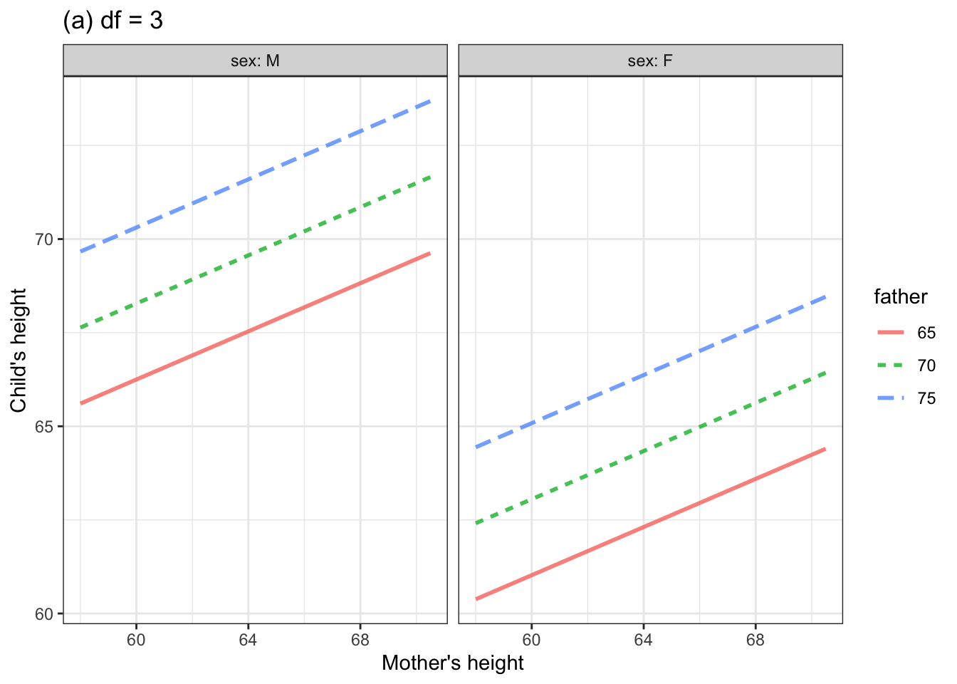
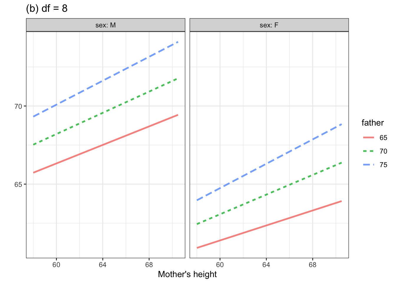
Figure 4. Two models of child’s height versus mother’s height. Father’s height and child’s sex are included as explanatory variables. Although father’s height is a quantitative variable, the graph shows the model for only three, evenly spaced, discrete values.

Comparing the two models, you might see how a larger \(\flex\) corresponds to increased flexibility.

You might also note from Figure 4 that the model with 8 degrees of freedom suggests that the taller is that father, the more influence the mother has on child’s height. The methods of statistical inference let us examine whether this claim is actually justified.

6.4 Flexibility, literally

Chapter 5 imagined a contest between two students, Linus and Curly, for the best model. Let’s return to that example, but now we’ll construct some models that are more flexible than a straight line.

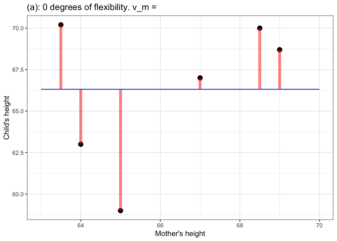
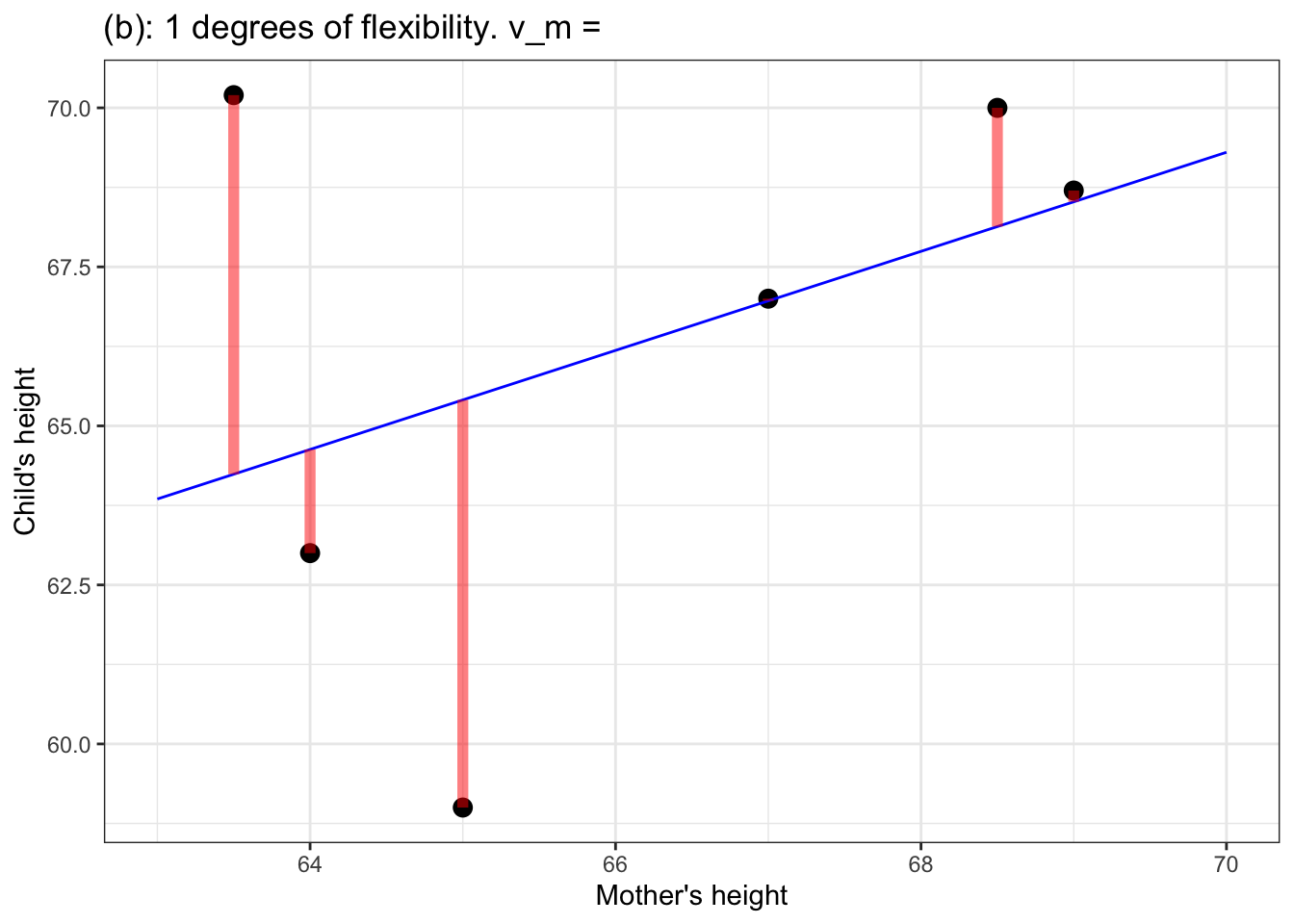
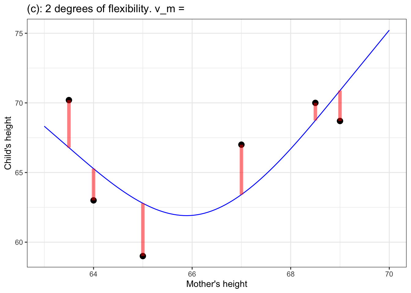
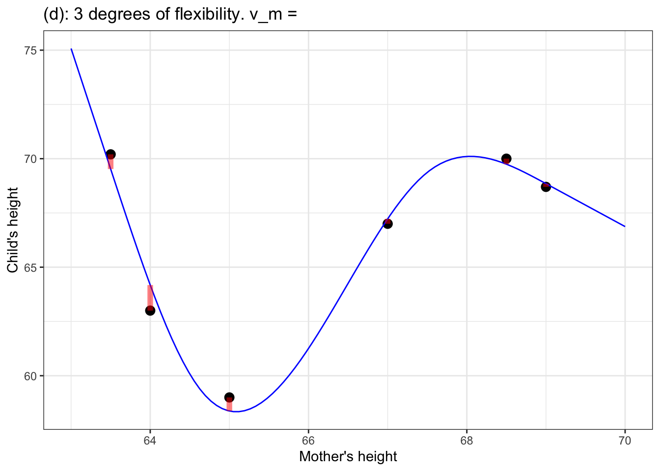
Figure 5: (a) a flat model – zero degrees of flexibility, \(\flex=0\); (b) a straight-line model – one degree of flexibility, \(\flex = 1\); (c) a model with one bend – two degrees of flexibility, \(\flex = 2\); (d) a model with two bends – three degrees of flexibility, \(\flex = 3\).

In the models in Figure 5, the degrees of flexibility indicate the shape of the function. A flat line has no degrees of flexibility. A sloped line has one degree of flexibility. Adding a bend adds another degree of flexibility, so 3 degrees of flexibility corresponds to two bends.

Notice that as the degree of flexibility goes up, the model function gets closer to the data points. Correspondingly, the variance of the model values, \(v_m\), goes up with increasing degrees of flexibility.

The point of counting degrees of flexibility is to be able to adjust \(v_m\) to take into account the intrinsic nature of flexibility to match more closely the response values. For sufficiently high degrees of flexibility, a model will be able almost perfectly to reproduce the response variable, even when there is no relationship between the response and explanatory variables.

6.5 Degrees of flexibility and freedom

The term “degrees of flexibility” is not at all conventional in statistics. I like “flexibility” because it gets at how curvy and complex and multivariate a model is. Flexibility is about the model itself. But the tradition in statistics is to use a quantity called the “degrees of freedom”–often written df–which takes into consideration the sample size \(n\). There is a very close relationship between df and \(\flex\):

\[\mbox{df} \equiv n - (1 + \flex) .\] I might just as well have written this book using df instead of \(\flex\), but I want to encourage you to think about how much flexibility a model has to help it get close to the data. For me, the sample size \(n\) plays a different role, as you’ll see in the next chapter.