Chapter 4 Modeling variation

The point of statistics is to understand how things vary. For instance, human height varies from one person to another. Some of that variation is associated with the sex of the person: women tend to be slightly shorter than men. Some of the variation in height relates to genes and genetic variation, some to differing nutrition and general health, etc.

Statistical models attempt to use the variation in explanatory variables – sex, genetic traits – to account for the variation in a response variable. To offer a contemporary example, some automobiles are involved in fatal accidents and some (the vast majority, thankfully!) are not. It varies. What’s behind the variation? It could be the weather conditions at the time. It also be human driver fatique, inebriation, incompetence, distraction, etc. It could also be characteristics of the vehicle itself: size, weight, maneuverability, breaking power, physical wear, automatic breaking, etc. And a lot of the variation is a matter of chance: for instance, the arrival of another car at an intersection at a particular instant.

4.1 Statistical models

For our purposes, a statistical model is a mathematical function that takes values of the explanatory variables as input and produces a corresponding output. For instance, a model of a person’s height might take the person’s age, sex, mother’s height and father’s height as inputs and give as output a specific number that we interpret as height. It might happen, by accident, that the model output is exactly on target for any particular person. More likely, though, the model output will be somewhat off: the person is somewhat shorter or taller than the model says. This is to be expected since the model can’t take into account every factor that influences height and because chance also plays a role.

4.2 Quantitative response variables

Consider the model (and data) shown in Figure 4.1. These are Galton’s records on the heights of adult children in London families. In Figure 4.1, height has been selected as the response variable. To keep the example simple, the role of explanatory variable has been assigned to sex. The statistical model takes as input a level of sex and produces as output a numerical value for the response variable.

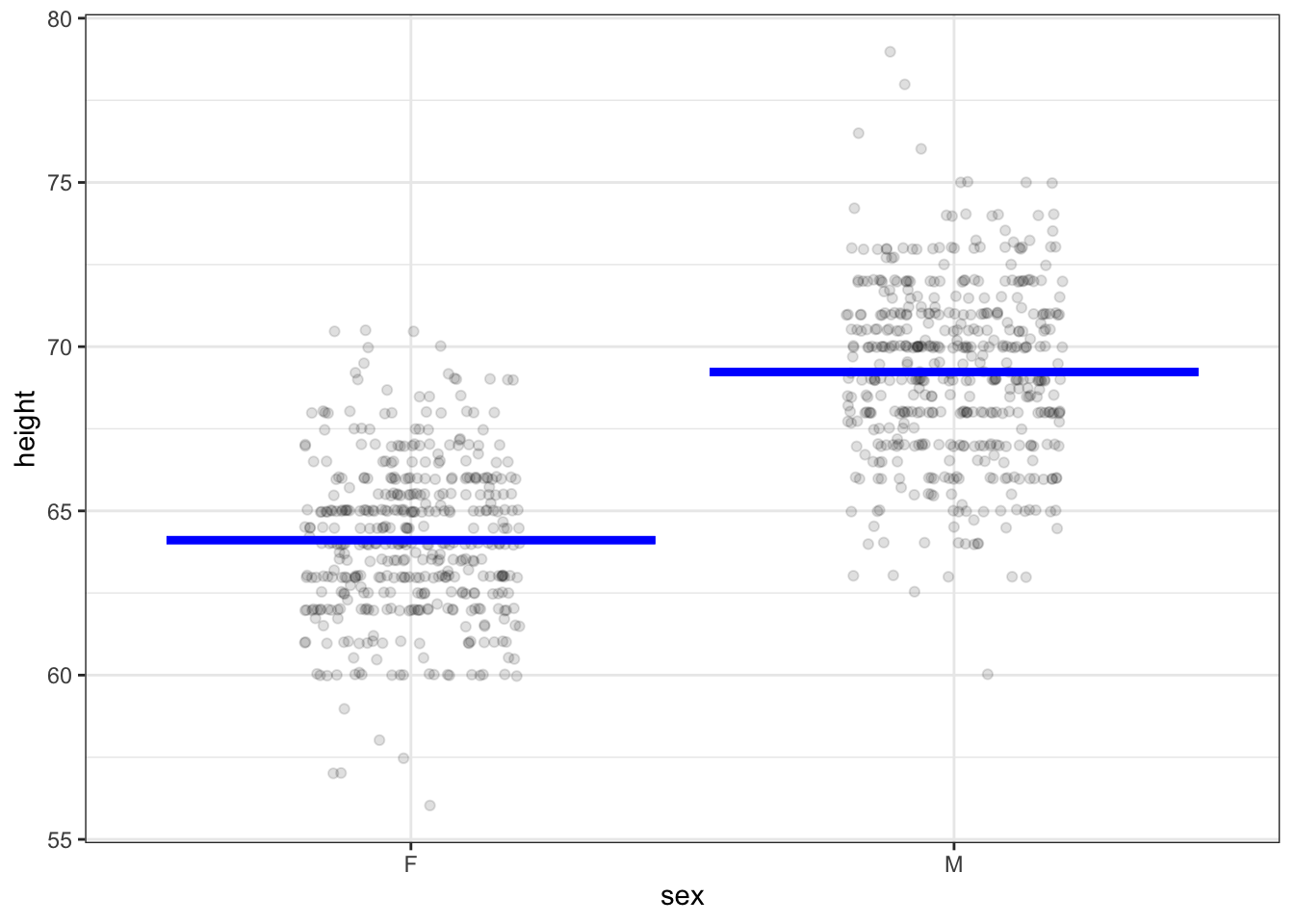
Figure 4.1: Galton’s height measurements with height as the response variable and sex as the explanatory variable. The model gives a single output for each level of the explanatory variable.

As you can see from Figure 4.1, the output of the model is about 64 inches when sex is F, and 69 inches when sex is M.

How are the model outputs determined? Or, in other words, what method is used to construct the model? The details will be covered in the next chapter. For now, the primary point is that the kind of model being shown describes the center of the distribution of individuals. A secondary point is that the model methodology is standard and automatic; the model outputs were established strictly using sex as the explanatory variable without consideration of anything else and without room for a human to manipulate the numbers or shade them into a preferred direction.

Galton was not directly interested in sex-related traits. His primary interest was in parent’s height as the explanatory variable. He recorded parent’s height quantitatively: a number. Figure 4.2 shows an example where the explanatory variable is numeric, as opposed Figure 4.1 which uses a categorical explanatory variable. The question that motivated Galton to collect the height data in the first place was to characterize the genetics of height: the extent to which it’s fair to say that a child inherits the height of his or her parents.

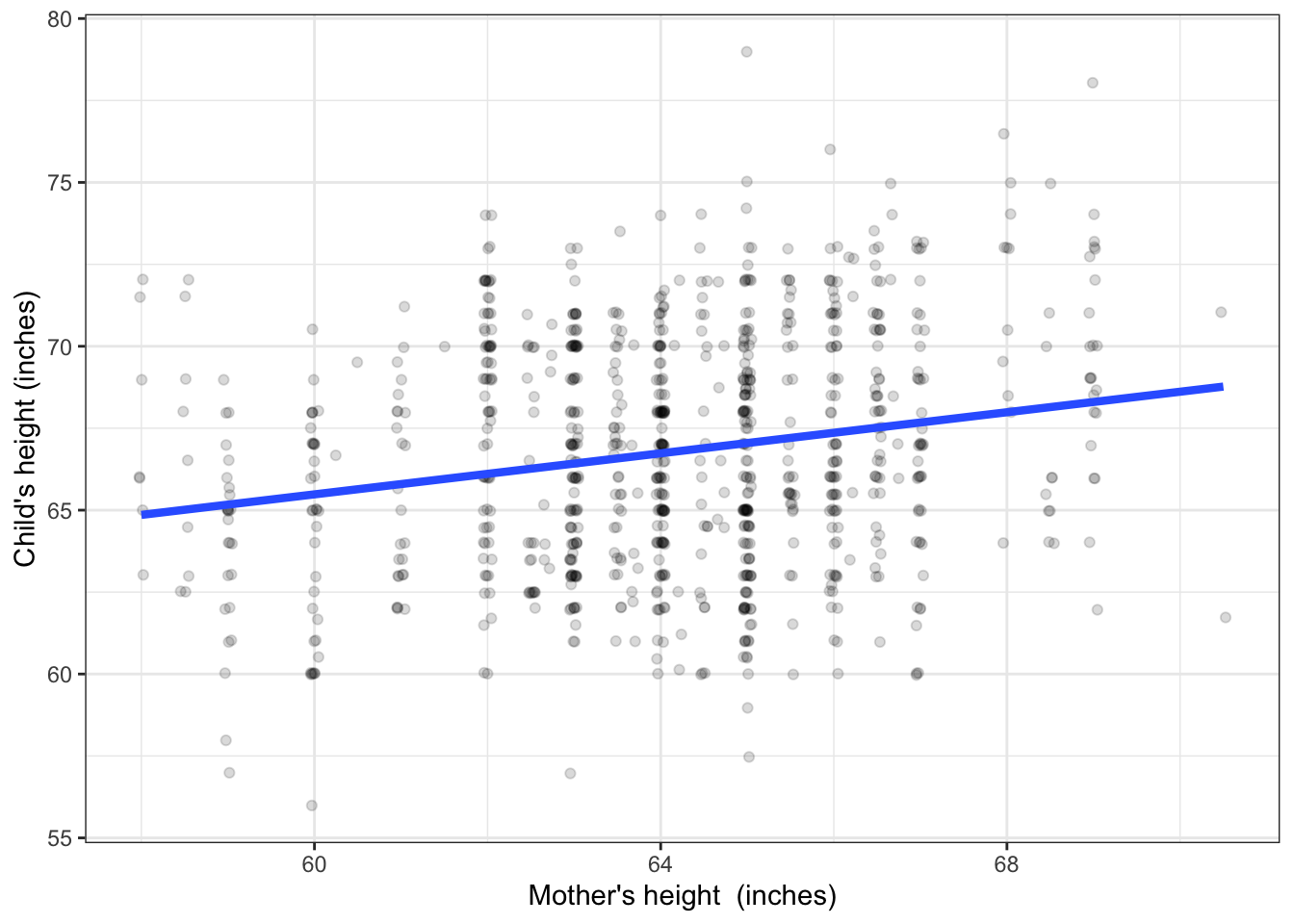
Figure 4.2: Child’s height versus the mother’s height. A conventional form of model is a straight line.

Consider first the model as a function. The input is the explanatory variable, mother’s height. The output is a number. So, for an input of 60 inches, the output is about 66 inches. For an input of 68 inches, the output is somewhat higher: about 68 inches.

The model output describes the center of the distribution of adult-child heights. That center is somewhat lower among the children of relatively short mothers than it is among the children of relatively tall mothers. Note that hardly any individuals exactly match the model output generated when the input is set to their mother’s height; almost all are either shorter or taller.

Some people mistakenly believe that the point of such a model is to predict the child’s height. Putting aside the question of why anyone would want to do this (perhaps you are wanting to buy a college graduation gown for your pregnant friend’s baby?), any meaningful prediction should be framed as an interval. So, for a 60-inch tall mother, a fair prediction would be for a child between 58 and 73 inches, while for a relatively tall 68-inch mother, the prediction would be 62 to 76 inches.

There is so much overlap in the prediction intervals for children of mothers of very different height that the model tells us almost nothing about individuals. But this is not the purpose of the model. Galton’s objective in collecting the data was to say how much of the variation in height is attributable to genetics. The conventional measure of how much, introduced in Chapter 8, is that mother’s height accounts for about 4% of the variation in height among children. Note that it’s 4% of the variation in height among children, not 4% of the height of an individual child.

Four percent doesn’t seem like much. Taking away the line in Figure 4.2 and looking just at the data points, you couldn’t fault someone for modeling the data with a level line, that is, one where the model output doesn’t change at all with mother’s height. One role of statistical inference is to answer the following question: Is there good reason to claim that the evidence provided by the data rule out a level-line model?

4.3 Proportions and indicator variables

The previous examples involved models where the response variable is numeric. In this section, we look at the special case of the numerical response variable being an indicator variable.

Recall that a single indicator variable can be used to encode a two-level categorical variable, for instance yes/no, alive/dead, succeed/fail, etc.

To illustrate, consider some data from another approach to quantifying genetics by experimental manipulation. This tradition started with Gregor Mendel in the 1860s, who famously cross-bred peas. Students of genetics know the name Mendel. Another famous name is Reginald Punnett (as in the Punnett square), whose cross-breeding work was done around 1905.

In one experiment, Punnett cross-bred sweet peas and observed the offspring’s flower color (binary levels white/other) and the shape of pollen granules (binary levels round/long). A few rows of data (translated to a modern format) from this experiment are shown in Figure 2.2 in Chapter 2. The complete data are graphed in Figure 4.3, below.

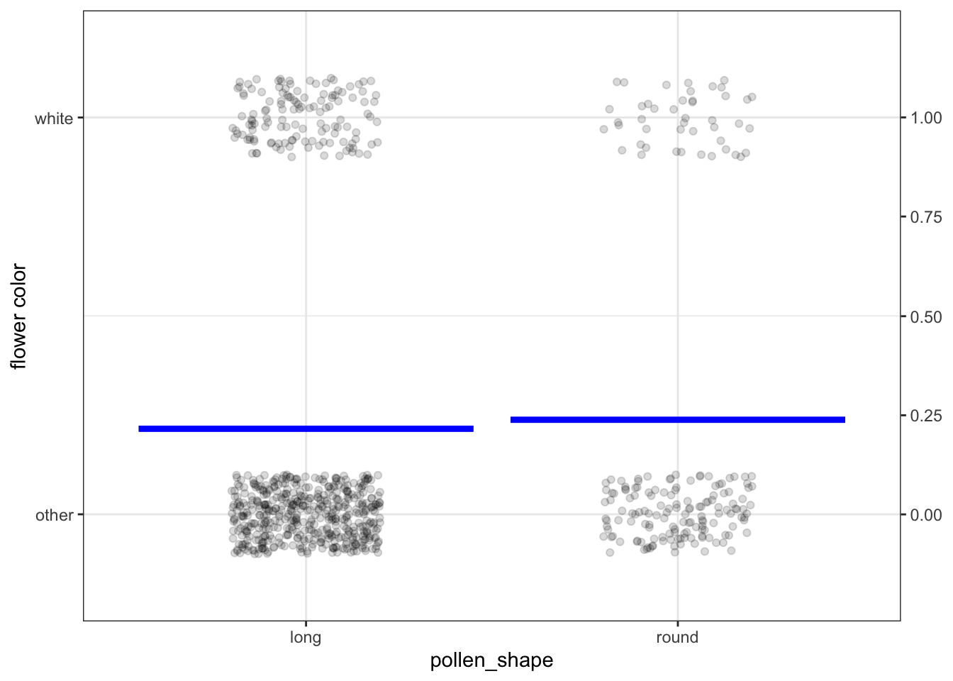
Figure 4.3: Punnett’s data from cross breeding peas, along with a model of flower color versus pollen shape.

There are only four possible combinations of white/other and long/round. To avoid plotting the rows directly on top of one another, the dots have been jittered. You can see that peas with “other” color and long pollen grains are the most common.

The model here is very similar to that of Figure 4.1. The response variable, flower color, has been translated into an indicator variable taking on only the values zero or one. The model provides an output for each level of the explanatory variable, pollen shape. Notice that the model output is not set in terms of white/other, but as a number between zero and one.

For models with an indicator response variable, the output is usually interpreted as a probability. For instance, when the pollen shape is long, the model output is 0.24. When the pollen is round, the model output is 0.25. We interpret a model output of 0.25–that is, 25%– as meaning that a quarter of the offspring will have white flowers. Comparing the model-output for long-pollen plants to that for round-pollen plants suggests that the probability of white flowers might be somewhat higher for round-pollen plants than long-pollen plants. The previous sentence uses some qualifying word: “suggests,” “might be,” “somewhat.” That’s to indicate that the statistical claim has not yet been vetted using the tools of statistical inference.

You can pretty much draw functions like this by hand if you keep in mind some simple rules. First, the function has to stay as close to the data as possible. Second, the function has to stay centered on the data.² It might help to understand the impact of these rules by comparing functions that do and don’t follow the rules. In Figures 4.3 and 4.4, the blue function follows the rules; the red ones do not.

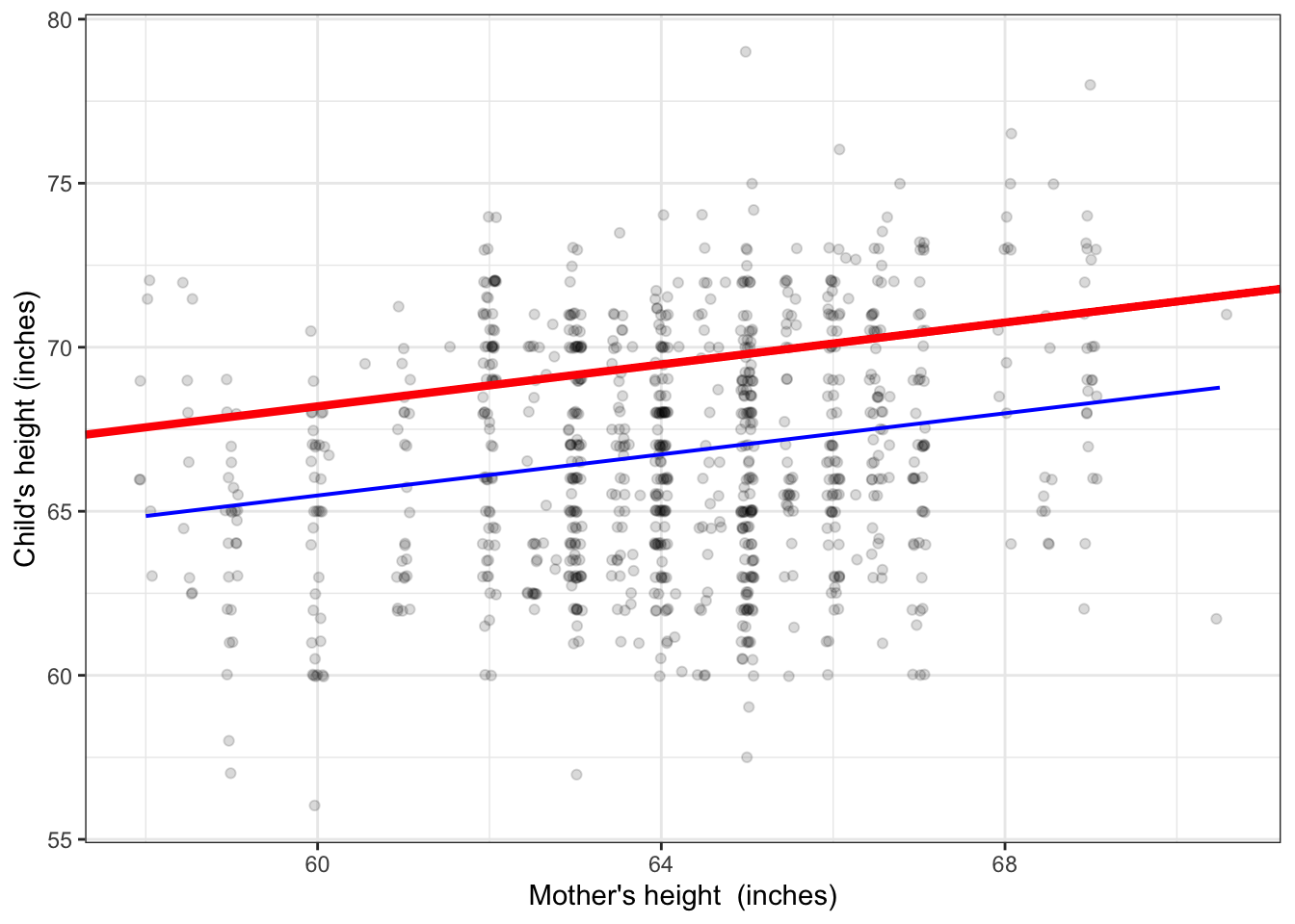
Figure 4.3: The red function is a bad match to the data. The large majority of points are far below the function. The blue function has the same form – a straight line – but is a legitimate match to the data, with data points more or less evenly balanced between being above and being below the blue line.

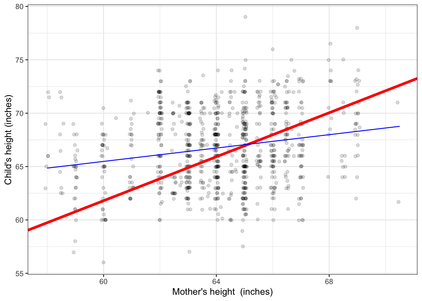
Figure 4.4: The red function is a bad match to the data. At heights below 63 inches, almost all the data points are above the red line.

Note that the blue functions in Figures 4.3 and 4.4 are centered in the sense that whatever value for the explanatory variable you look at, the data points are just about evenly distributed above and below the function. The red functions don’t accomplish this.

4.4 A taxonomy of simple models

Recall that the response variables covered in this book are quantitative, which includes both regular numerical variables (like height) and indicator variables (like that for sex). Explanatory variables can be either quantitative or categorical. This suggests that models with one response and one explanatory variables fall into one of four types:

Setting	response variable	explanatory variable	Figure	conventional name
1	quantitative	categorical	4.1	groupwise means / t test
2	quantitative	quantitative	4.2	linear regression / slope test
3	categorical (indicator)	categorical	4.3	groupwise proportions / p test
4	categorical (indicator)	quantitative	4.5	not usually included in introductory statistics

Figures 4.1, 4.2, and 4.3 show the first three settings. Figure 4.5 shows the fourth setting, a categorical response variable and a numerical explanatory variable.

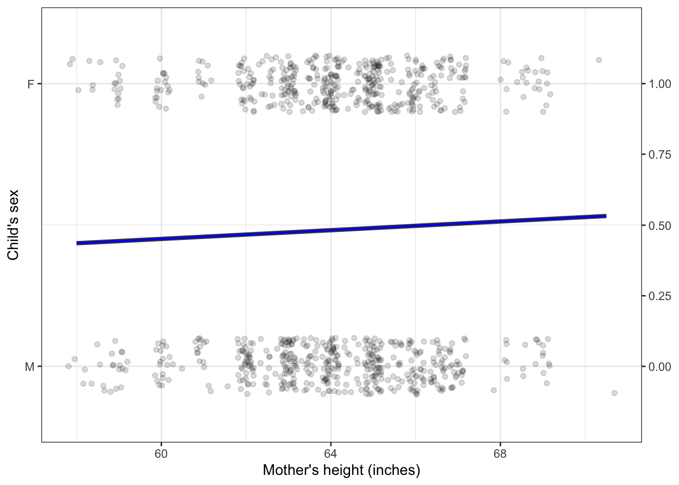
Figure 4.5: A model with an indicator response variable and a numerical explanatory variable.

Again, the model output is numeric, in the form of the probability that the child is female. The model suggests that 60-inch tall mothers are slightly less likely to bear girls and 68-inch tall mothers. Common sense suggests that a baby’s sex is not influenced by the mother’s height. Correspondingly, the model output is around 50% regardless of the mother’s height.

Perhaps you’re surprised to see that there is any slope at all to the function. Don’t be surprised yet, because we haven’t shown that such a statement is justified by the data: we have a setting for inference but have not yet carried out the inference calculations to tell us if the statement is justified.

For purposes of inference, conventional texts treat settings 1, 2, and 3 as different. (They don’t handle setting 4 at all.) I’ve added to the table the conventional name assigned to the different inferential tests in each setting.

But in all settings, exactly the same technique, called linear regression, has been used to match the model to the data.³ In this book, rather than introduce four different inferential procedures, we’ll have just one. That’s a major factor behind the ability to describe classical inference concisely.