Chapter 9 Confidence intervals

\(\newcommand{\flex}[]{^\circ\!{\cal{F}}}\)

Chapter 7 started with an example of an effect size: the reduction in risk of fatal injury of vehicle occupants with respect to wearing a seat belt. That reduction is pretty impressive: about 58% according to a report (Kahane 2017) from the US National Highway Traffic Safety Administration (NHTSA).

This chapter deals with the word “about” in the previous sentence. “About” is a statement about the precision of the effect size: how well we know it. It’s natural–but wrong–to assume that the precision can be sorted out from the effect size itself. For 58%, common sense suggests that about means something like “in the range from 56% to 60%.”

In fact, the report (Kahane 2017) explicitly states the precision as 41% to 69%. The format of this statement is an interval, the “confidence interval” on the effect size of risk reduction with respect to wearing a seat belt.

9.1 Calculating confidence intervals on effect size

Conventional textbooks have dozens of pages covering the calculation of confidence intervals for the four settings introduced in Chapter 4. Each of those settings involves a single explanatory variable and \(\flex = 1\). We can simplify a bit. The steps are:

1. Find the effect size itself, using the techniques in Chapter 7. We’ll call the effect size B and it will be a slope or a difference depending on whether the explanatory variable is quantitative or categorical.
2. Find the F statistic for the model.
3. Calculate the confidence interval (CI) on the effect size.

Being an interval, a confidence interval is a range of values delimited by a lower and upper bound. But it’s common to display the interval using plus-or-minus \(\pm\) notation. In \(\pm\) notation, the confidence interval on the effect size is written

\[\mbox{B} \pm \mbox{margin of error}\]

We already know B. The margin of error has a very simple formula involve both B and F:

\[\mbox{margin of error} = \mbox{B}\sqrt{4 / \mbox{F}}.\] Example: For the model shown in Figure 7.1, the effect with respect to sex of child’s height is found to be \(B = 5.1\) inches. The F statistic is 933. So the margin of error on the effect size is
\[5.1\ \mbox{inches}\sqrt{4/933}\ \ \ \approx\ \ 0.33\ \mbox{inches}\]

Correspondingly the confidence interval will be:

\(5.1 \pm 0.33\) inches, or, 4.77 to 5.43 inches

Example: For the model shown in Figure 7.2, the effect of child’s height with respect to mother’s height is found to be B = 0.31. The F statistic is 34. So the margin of error is

\[\mbox{margin of error} = 0.31 \sqrt{4/34}) \approx 0.11\] The confidence interval itself is

\[0.31 \pm 0.11\ \ \ \mbox{or}\ \ \ 0.20\ \mbox{to}\ 0.42\] This simple method for finding the confidence interval on an effect size works only when \(\flex = 1\). For models with multiple explanatory variables, confidence intervals can be calculated, but not with this simple formula. A formula can be expressed using concepts from linear algebra, but in practice everyone relies on statistical software to do the calculations.

9.2 4 and 95%

The confidence intervals described above are called “95% confidence intervals.” The 95% is called the “confidence level.” A precisely mathematical interpretation of that 95% is difficult for many people to follow and easy to get wrong.⁵ It suffices to say two things:

1. 95% is the conventional confidence level, so use it.
2. It’s common to hear this interpretation of the 95% confidence interval: “95% of the time, the true value of the effect size will be inside the interval.” This is not exactly right, in part because we would need to know what “true” means in order to operationalize the statement. But, even if the interpretation is not right, it gives a reasonable impression of the intent behind a 95% confidence interval.
3. There is a small group of people who need to figure out how to calculate confidence intervals. For these people, it’s important to know exactly what a confidence interval is intended to mean. You’ll see the play out in the following explanation, which attempts to show how we know the formula for the CI produces an interval at a 95% confidence level.

Notice that in the formula for the 95% margin of error on the effect size \[\mbox{margin of error} = B \sqrt{4/F}\] the number 95% does not directly appear. What is it about this formula that makes the margin of error at a 95% confidence level rather than some other level? It is the number 4, which can be seen as the result of an experiment.

Here’s the experiment. Make some data where the variables are composed entirely of random numbers. It doesn’t really matter what the sample size \(n\) is. For now, let’s assume \(n \gtrapprox 25.\) Pick one of the variables as a response–it doesn’t matter which one. Then pick others as the explanatory variables–again, it doesn’t matter much which ones or how many. Let’s say you use \(\flex\) of them, where you get to choose \(\flex\).

Since we are making up the data, we know exactly the mechanism that is generating it, so we are in a good position to say what’s “true” about the mechanism. Since the response and every explanatory variable are random, the “true” effect size with respect to any of the explanatory variables is zero.

Now construct a model of the response variable as a function of the explanatory variables, find the variance \(v_r\) of the response variable and the variance \(v_m\) of the model values. Use these along with \(n\) and \(\flex\) to find the F for the model. Since there is no connection between the response and the explanatory variables, we expect F to be small. Indeed, the typical F found by such an experiment is the very definition of “small” for F. Small F means that the random number variables hypothesis is consistent with the data seen through the lens of our model.

Since the F from the experiment was generated using random numbers and random choices of variables and \(\flex\) and \(n\), the F value is itself random.

Now imagine that you repeat the experiment over and over with different random data, different choices of variables, and different \(\flex\). Remarkably, you will find a distribution of F that is centered more or less at 1 and which falls off with larger F. About 95% of the experimental trials, it turns out, will have \(F < 4\).

Look again at the formula for the margin of error on the effect size, \[\mbox{margin of error} = B \sqrt{4/F}\] When \(F < 4\), which happens 95% of the time, the confidence interval quantity under the radical, \(\sqrt{4/F}\) will be greater than 1. So the margin of interval has a magnitude larger than B itself, meaning that the confidence interval must include zero. Thus, when the “true” effect size is zero, as implemented by the random generation of data, the confidence interval constructed using 4 as the number in \(\sqrt{4/F}\) will include zero 95% of the time. That’s exactly what we want a confidence interval to do.

9.3 4 and \(n\)

Very precise calculations of the 95% level of F for models fitted to completely random data can be made using advanced mathematics. Of course, such calculations make assumptions about the mechanism generating the random data, which is to say that the calculations are precise only in a specific made-up world. Calling this the “official” standard for the random data world, we can say that officially, the 95% level of F varies somewhat with the sample size \(n\) and the model flexibility \(\flex\).

This chapter is about confidence intervals on effect sizes from the single explanatory variable in models with \(\flex = 1\), so let’s focus on how official F varies with \(n\) when \(\flex = 1\).

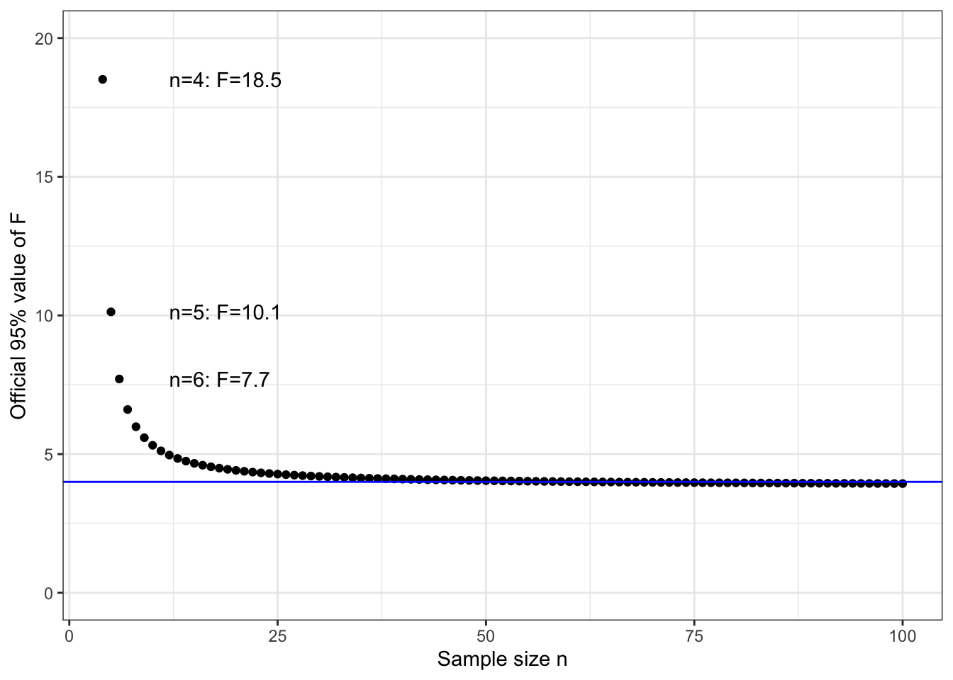
Figure 9.1: The official 95% values of F to be used in confidence interval calculations are a function of \(n\). The blue line marks the value of 4, which is a good match to the official value when \(n > 10\).

Let’s use the symbol \(F^\star\) to label the “official” 95% values for F. An improved formula for the margin of error of an effect size (when \(\flex = 1\)) is

\[\mbox{margin of error} = B \sqrt{F^\star/F} .\]

For a teacher, it’s worth asking whether to teach the “improved” formula first, or at all. One perspective is that it’s trivial to find \(F^\star\)–just read it off the graph. So why not used the improved formula?

There are a few reasons. First, every step in a procedure imposes some cognitive load on students which distracts them from other matters. Second, \(F^\star\) doesn’t explain anything. The explanation of 4 is challenging enough and likely to be understood only by a small fraction of students (unless you spend time doing the simulation). But hardly any math or statistics faculty understand the origins of \(F^\star\) and for students it’s just another mystery. Statistics calculations are always done in practice using software, so \(F^\star\) is automatically included in the computation. More important, there is are issues that make the details of \(F^\star\) relatively unimportant: the choice of measures, the shapes of distributions, and the role of covariates.

Insofar as a desire to cover the details of \(F^\star\) causes the instructor to use very small \(n\) in examples, the statistics course is being pushed in bad direction. It’s much more important, in today’s world of data, to show how statistics can be applied to realistic problems, which always involve covariates. If you want to teach a unit on “small data,” do that. But it probably won’t be very interesting.

9.4 Confidence versus prediction intervals

One of the common mistakes made by students in introductory statistics is to confuse a confidence interval with a prediction interval. For example, consider a confidence interval on the mean commuting time for workers in a city, say 35 to 42 minutes. Experience shows many well educated people will mistake this for a prediction of how long a person’s commute takes, that is, that 95% of people have commuting times in the range 35 to 42 minutes.

It’s entirely possible to construct a proper prediction interval. It will typically involve a term in the form of \(\pm \sqrt{4 (v_r - v_m)}\), which, you should note, does not depend on \(n\). For large \(n\), the range \(\pm \sqrt{4 (v_r - v_m)}\) is typically the biggest determinant of a prediction interval.

9.5 For the conventionally trained reader …

The conventionally trained reader likely encountered confidence intervals in one of two settings: the CI on the sample mean or the CI on the sample proportion. Relatively simple formulas were presented for the standard error and then the standard error was scaled up by \(t^\star\) or \(z^\star\) to get a confidence interval. We’ll get to CIs on means and proportions in terms analogous to those used in this chapter only Chapter 11. The reason for the delay is that means and proportions are not effect sizes and that there is a mathematical difficulty using the formula for F when \(\flex = 0\).

Anticipating Chapter 11 here, a 95% margin of error for a mean or proportion is

\[\mbox{margin of error} = \sqrt{4 v_r / n}\] where \(v_r\) is the variance of the variable involved. (For proportions, of course, the variable is an indicator: the mean of an indicator is exactly the proportion of 1s in the indicator.)

Recognizing that the \(\sqrt{v_r}\) is the standard deviation \(s_r\), we get a formula that is likely more familiar to experienced instructors:

\[\mbox{margin of error} = 2 s_r / \sqrt{n}\]

References

Kahane, CJ. 2017. “Fatality Reduction by Seat Belts in the Center Rear Seat and Comparison of Occupants’ Relative Fatality Risk at Various Seating Positions.” DOT HS 812 369. US National Highway Traffic Safety Administration. https://crashstats.nhtsa.dot.gov/Api/Public/ViewPublication/812369.pdf.