Chapter 8 F and R

$\newcommand{\flex}[]{^\circ\!{\cal{F}}}$

We now have the pieces we need to assemble the central quantity which informs statistical inference. These are:

$n$, the sample size (or, more concretely, the number of rows in out data frame)
$v_r$, the variance of the response variable. $v_r$ for binary categorical response variables is based on the 0-1 encoding.
$v_m$, the variance of the model values.
$\flex$, the degree of flexibility.⁴

We’ll put these together to form a quantity called F.

8.1 The F statistic

The name, F, is in honor of Ronald Fisher, one of the leading statisticians of the first half of the 20th. The formula for F is pretty simple, so I’ll present it right here for ready reference.

\[F \equiv \frac{n - (1 + \flex)}{\flex} \frac{v_m}{v_r - v_m}\] For almost all the settings considered in introductory statistics courses, $\flex$ is 1, so the formula simplifies to: \[F = (n-2) \frac{v_m}{v_r - v_m}\] Example: Figure 4.1 shows a model of child’s height with respect to sex. The variance of the response variable (child’s height) is $v_r =$ 12.84 inches². The variance of the model values is $v_m =$ 6.55 inches². The data used to construct the model have $n = 898$, giving

\[F = 896 \frac{6.55}{12.84-6.55} \approx 897 \times 1.04 \approx 934 .\]

8.2 What’s the meaning of F?

F combines the four quantities $n$, $v_r$, $v_m$, and $\flex$. To get a notion why the combination works, keep these basic ideas in mind concerning what it means to have “more evidence.”

The larger $n$, the more evidence. That’s why F is more-or-less proportional to $n$. (Strictly speaking, F is proportional to $n - (\flex + 1)$.)
The more complicated the model – e.g. the number of explanatory variables or levels in an explanatory categorical variable – the less evidence. Or, put another way, we would want more evidence from data to justify a complicated model than a simple model. The division by $\flex$ in the formula for F implements this idea.
The closer the model values come to capturing the actual response variable, the greater the evidence that there is a relationship. An obvious way to quantify this closeness are with the difference $v_r - v_m$. We want the size of F to increase as $v_m$ gets closer to $v_r$. So F is proportional to $\frac{1}{v_r - v_m}$.
But the numerical value of the difference $v_r - v_m$ depends on the units in which the response variable is measured. For instance, we could express the running times in Chapter 1 in minutes or in seconds. But the difference $v_r - v_m$ would be $60^2 = 3600$ times larger if we used seconds than minutes. Obviously we don’t want our F value to depend on the units used. To avoid that, we divide $v_r - v_m$ by $v_m$, getting the $v_m / (v_r - v_m)$ in the formula for F.

8.3 R-squared

Many people prefer to look at a ratio $v_m / v_r$ to quantify how close the model values are to the values of the response variable. If the model does a good job accounting for the response variable, then $v_m$ will be close to $v_r$. That is, the ratio will be close to 1. On the other hand, if the model tells us little or nothing about the response variable, $v_m$ will be close to zero and the ratio itself will be zero.

The ratio has a famous name: R-squared, that is:

\[R^2 = v_m / v_r\] A more obscure name for $R^2$ is coefficient of determination, which is awkward but does express the point that $R^2$ is about the extent to which the explanatory variables, when passed through the model, determine the response variable. $R^2$ is, literally, the faction of the variance of the response variable that has been captured by the model.

$R^2$ can never be bigger than one and can never be negative. When $R^2 = 1$, the model values are exactly the same as the values of the response variable.

When there is no connection between the r esponse and explanatory variables, $R^2$ will be small. Ideally, it would be zero, but the process of random sampling generally pushes it a little away from zero. One way to think about F is as indicating when there is so little data that a small but non-zero R² is consistent with the hypothesis that there is no connection between the response and explanatory variables.

Example: Figure 4.1 shows a model of child’s height with respect to sex. The variance of the response variable (child’s height) is 12.84 inches². The variance of the model values is 6.55 inches². Thus: \[R^2 = 6.55 / 12.84 = 0.51 = 51\%\]

8.4 F in statistics books

In most statistics book, F is not written in the form above but in one of a couple of alternative – but equivalent – forms. There’s no particular reason to use these forms. Knowing what they look like will help you make sense of traditional statistical reports.

Since $R^2$ summarizes the relationship between $v_m$ and $v_r$, the formula for F can be written in terms of $R^2$. This is the first of the alternative forms.

\[F = \frac{n - (\flex+1)}{\flex} \frac{R^2}{1 - R^2}\]

Another alternative form comes from using an intermediate in the calculation of $v_m$ and $v_r$. Recall how the variance is calculated by calculating square differences and averaging. To average, of course, you add together the quantities and then divide by the number of quantities being averaged.

Suppose you didn’t bother to average, and stopped after adding up the square differences. The name for this intermediate is the sum of squares. F is often written in terms of the sum of squares of the response variable SS_r_ and of the model values SS_m_. Something like this:

\[F = \frac{n - (\flex+1)}{\flex} \frac{\mbox{SS}_m}{\mbox{SS}_r - \mbox{SS}_m}\]

More typically, instead instead of looking at the model values directly, the tradition in classical inference is to consider what’s called the sum of squares of the residuals, which is simply SSR = $\mbox{SS}_r - \mbox{SS}_m$ and the formula is re-written like this:

\[F = \frac{\mbox{SS}_m / \flex}{SSR / (n - (\flex + 1))}.\] Both the numerator and the denominator of this ratio have the form of a sum of squares divided by a count. In the terminology of classical inference, such things are called mean squares.

In this book, we’ll just use the formula for F given at the start of this chapter. The others give exactly the same value, but let’s avoid having ton work with potentially confusing vocabulary such as the mean square and sum of squares.

8.5 Another explanation of F

First, I’ll give the explanation in the form of a parable. Imagine that your model is a automobile. You are going to drive it a distance of 100 miles. There are two gas companies, EXPLANATORY Fuel and RANDOM Fuel. You put in 2 liters of EXPLANATORY gas and drive as far as you can get, say 44 miles. Your fuel economy on the EXPLANATORY part of the trip is thus 22 miles per liter. You’re out of fuel, but conveniently there is a RANDOM gas station close at hand. You fill up your tank with RANDOM gas and continue driving. You drive the rest of the way using the random gas. Looking at the fuel gauge, you see that you have used up 8 liters of RANDOM gas, the fuel economy is 56 miles (that is, 100-44) per 8 liters of RANDOM gas, so the fuel economy is only 7 miles per gallon of RANDOM gas.

Now a skeptic asks you, “The EXPLANATORY gas company has a good name for marketing, but do you have any good reason to think that EXPLANATORY gas is better than RANDOM gas?” Of course, the answer is yes, but how to summarize your findings? One way is to compare the fuel economies of the different kinds of gas: 22 miles per gallon for EXPLANATORY and 7 for RANDOM. More concisely, you could say that EXPLANATORY gas is more than 3 times (22/7) as efficient as RANDOM gas.

The miles travelled using EXPLANATORY gas corresponds to R². The fuel itself is whatever explanatory variables (and nonlinearities and whatever) are in your model. The amount of EXPLANATORY gas is $\flex$.

RANDOM gas is not manufactured from genuine explanatory variables. Instead it is synthesized purely from random numbers. You don’t expect RANDOM gas to be very good. But it serves as a point of comparison for the effectiveness of EXPLANATORY gas.

To conduct the comparison, you’ll look at the ratio of the fuel economies: EXPLANATORY fuel economy divided by RANDOM fuel economy. That ratio of fuel economies corresponds exactly to F.

Perhaps you’re thinking, “RANDOM gas won’t get you anywhere.” That’s not true. You can confirm this by creating a dataset that consists only of random numbers then modeling one of the variables by the others. You’ll find that R² is not zero. Indeed, if you use $n-1$ random explanatory variables in your model, you’re guaranteed to reach $\mbox{R}^2 = 1$.

Figure 6.13 shows simulations of R² versus $\flex$ for RANDOM gas. (Not every gallon of RANDOM gas is the same, it’s random!)

(ref:R-path-cap) Figure 6.13: The dark path shows one trial in which the car is fueled entirely with RANDOM gas. The graph shows how far the car gets (in terms of R²) as it uses more and more fuel (in terms of $\flex$).

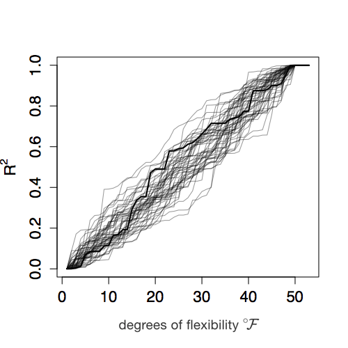
Figure 8.1: (ref:R-path-cap)

Figure 6.14 shows schematically the general form of distance R² versus fuel consumption when the first 10 units of fuel (that is to say, $\flex = 10$) are EXPLANATORY gas. As you can see, the EXPLANATORY gas got you to R² = 65%. So the fuel economy for EXPLANATORY gas is about 6.5% per unit of fuel.

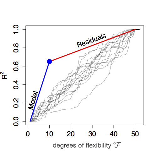
$Figure 6.14: $\mbox{R}^2$ versus $\flex$. For the first 10 units of fuel, EXPLANATORY gas was used. Then the car switched over to RANDOM fuel for the rest of the journey to $\mbox{R}^2 = 1$. Note that the path upward to the blue dot (using EXPLANATORY gas) is much steeper than for the rest of the journey using RANDOM gas. The slope of each segment is the fuel economy.$

Figure 8.2: Figure 6.14: $\mbox{R}^2$ versus $\flex$. For the first 10 units of fuel, EXPLANATORY gas was used. Then the car switched over to RANDOM fuel for the rest of the journey to $\mbox{R}^2 = 1$. Note that the path upward to the blue dot (using EXPLANATORY gas) is much steeper than for the rest of the journey using RANDOM gas. The slope of each segment is the fuel economy.

With enough RANDOM gas, you’ll get the rest of the way to R² = 100%. How much is enough? $n - (\flex + 1)$ units of fuel. Since $n=50$ and $\flex = 10$, the RANDOM gas fuel economy is 35% (that is, 100% - 65%) divided by 39, or just under 1% per unit of fuel. The F statistic is therefore 6.5% / 1% = 6.5.

Is 6.5 a big enough F to convince us that the EXPLANATORY gas is clearly not just RANDOM gas in disguise? We can find that out by doing a simulation where we use only RANDOM gas in the car, comparing how far we get with the first $\flex = 10$ liters to how much addition RANDOM fuel to get to our eventual destination of R² = 100%. That’s what Figure 6.13 is about. You can mark on any of those random paths the value of R² reached with the first $\flex = 10$ liters of fuel. Then draw in the equivalent of the blue slope and the red slope. For the large majority of trials, the ratio of slopes will be less than 4. So $F = 6.5$ is not a plausible outcome when using only RANDOM fuel in the car.

Note the expression for F in terms of R²:

\[F \equiv \frac{\mbox{R}^2}{\flex} \div \frac{1 - \mbox{R}^2}{n - (\flex + 1)}\]

The first ratio in the above is the slope of the blue line segment in Figure 6.14. The second ratio in the above is the slope of the red line segment in Figure 6.14.