Topic 2 Notes

2.1 Review of Day 4, Sept 15, 2017

How the linear regression architecture relates to machine learning.
- linear regression is designed to work even in “small data” situations where
  1. cross-validation is not appropriate
  2. the number of model degrees of freedom may be almost as large as $n$
- provides a ready definition of the “size” of a model: the number of coefficients.
Main software used in linear regression, lm() and predict()
Programming basics: indexing of vectors, matrices and data frames.

2.2 Regression and Interpretability

Regression models are generally constructed for the sake of interpretability:

Global linearity
Coefficients are indication of effect size. The coefficients have physical units.
Term by term indication of statistical significance

An example on College data from ISLR package

data(College, package="ISLR")
College$Yield <- with(College, Enroll/Accept)
mod1 <- lm(Yield ~ Outstate + Grad.Rate + Top25perc, data = College)
mosaic::rsquared(mod1)

## [1] 0.2170221

mod2 <- lm(Yield ~ . - Grad.Rate, data = College)
mosaic::rsquared(mod2)

## [1] 0.5004599

What variables matter?
How good are the predictions?
How strong are the effects?

2.3 Toward an automated regression process

In machine learning, we ask the computer to identify patterns in the data.

In “traditional” regression (which is still very important), we specify the explanatory terms and the computer finds the “best” model with those terms: least squares.
In machine learning, we want the computer to figure out which terms, of all the possibilities, will lead to the “best” model.

2.4 Selecting model terms

The regression techniques

Traditional regression:
- Our knowledge of the system being studied.
- Heirarchical principal
  - main effects, then
  - interaction.
Machine learning
- Look at all combinations of variables?
- Activity 1:
  - Write a statement that will pull 2 random variables from a data frame and the explanatory variable.
  - Use Yield ~ . as the formula.

explanatory_vars <- names(College)[-19]

my_vars <- sample(explanatory_vars, size = 12)
new_data <- College[ , c(my_vars, "Yield")]
mod <- lm(Yield ~ ., data = new_data)
mosaic::rsquared(mod)

## [1] 0.4844153

mod

## 
## Call:
## lm(formula = Yield ~ ., data = new_data)
## 
## Coefficients:
## (Intercept)     Outstate       Accept  F.Undergrad       Expend  
##   5.811e-01   -9.815e-06   -6.451e-05   -5.232e-06    3.157e-06  
##  Room.Board          PhD     Terminal       Enroll    S.F.Ratio  
##  -1.565e-05   -8.138e-04   -2.090e-04    1.877e-04    2.209e-03  
##   Top10perc  perc.alumni   PrivateYes  
##   9.096e-04   -4.334e-04    5.082e-03

2^18

## [1] 262144

Activity 2: * How many combinations are there of $k$ explanatory variables? Calculate this for $k = 5, 10, 15, 20$. How many are there in the College? * What about with interactions?
How long does it take to fit a model?

system.time( do(1000) * lm(Yield ~ ., data=College))

##    user  system elapsed 
##   6.468   0.051   6.594

256*7/3600

## [1] 0.4977778

names(College)

##  [1] "Private"     "Apps"        "Accept"      "Enroll"      "Top10perc"  
##  [6] "Top25perc"   "F.Undergrad" "P.Undergrad" "Outstate"    "Room.Board" 
## [11] "Books"       "Personal"    "PhD"         "Terminal"    "S.F.Ratio"  
## [16] "perc.alumni" "Expend"      "Grad.Rate"   "Yield"

With $k$ explanatory variables, $2^k$ possibilities, not even including interactions. Including first-order interactions, it’s $2^k + 2^{k(k-1)/2}$. Calculate this for $k=3. - Increase in $R^2$? Problem: $R^2$ will always go up as we add a new term. - Some other measure that takes into account how much $R^2$ should go up.

2.5 Programming basics: Graphics

plot(1, type = "n", xlim = c(100,200), ylim = c(300,500))

Basic functions:

Create a frame: plot(). Blank frame: plot( , type="n")
- set axis limits,
Dots: points(x, y), pch=20
Lines: lines(x, y) — with NA for line breaks
Polygons: polygon(x, y) — like lines but connects first to last.
- fill
Color, size, … rgb(r, g, b, alpha), “tomato”

2.6 In-class programming activity

Programming Activity 4: Drawing a histogram.

2.7 Day 5 Summary

2.7.1 Linear regression

Discussed “interpretability” of linear models, e.g. meaning of coefficients, confidence intervals, R^2, etc.
- which variables are “important” via ANOVA and mean sum of squares
Discussed metrics to compare models
- R^2 – not fair, since “bigger” models are always better
- Punishment: Two criteria for judging
  - R^2
  - How big the model is.
  - These two are somehow combined together into “adjusted R^2.” We’ll say more about that today.
- Cross-validation. Judge each model on its “out of sample” prediction performance.

2.7.2 Coefficients as quantities

Coefficients in linear models are not just numbers, they are physical quantities with dimensions and units.

Dimensions are always (dim of response)/(dim of this term)
The model doesn’t depend on the units of these quantities. The units only set the magnitude to the numerical part of the coefficient, but as a quantity a coefficient is the same thing regardless of units.
Conversion from one unit to another by multiplying by 1, but expressed in different units, e.g. 60 seconds per minute, 2.2 pounds per kilogram.

2.8 In-class programming activity

Day 5 activity

Drawing a histogram.

2.9 Day 6 Summary

$R^2$
- var(fitted) / var(response)
- partitioning of variance:
  - var(fitted) + var(resid) = var(response)
  - same with sum of squares: SS(fitted) + SS(resid) = SS(response)
Adjusted $R^2$
- $R^2$ vs $p$ picture
- Derive a formula from the picture: we’ve got $p+1$ df to get from $R^2 = 0$ to our observed $R^2$, so $n - (p+1)$ df left for the residuals. Rate of increase due to junk is $(1 - R^2) / (n - p - 1)$. Projecting back $p$ terms gives an adjustment of $(1 - R^2) / \frac{p}{n - p - 1}$. Subtract this from $R^2$.
- Wikipedia gives two formulas:
  - $Adj R^2 = {1-(1-R^{2}){n-1 \over n-p-1}}$ – this projects back $n-1$ terms from 1.
  - $Adj R^2 = {R^{2}-(1-R^{2}){p \over n-p-1}}$ — projects back $p$ terms from $R^2$.
Adjusted $R^2$
Whole model ANOVA.
ANOVA on model parts

2.10 Measuring Accuracy of the Model

$R^2$ = Var(fitted)/Var(response)
Adjusted $R^2$ - takes into account estimate of average increase in $R^2$ per junk degree of freedom
Residual Standard Error - Sqrt of average square error per residual degree of freedom. The sqrt of the mean square for residuals in ANOVA.

2.11 Bias of the model

You need to know the “truth” to calculate the bias. We don’t.

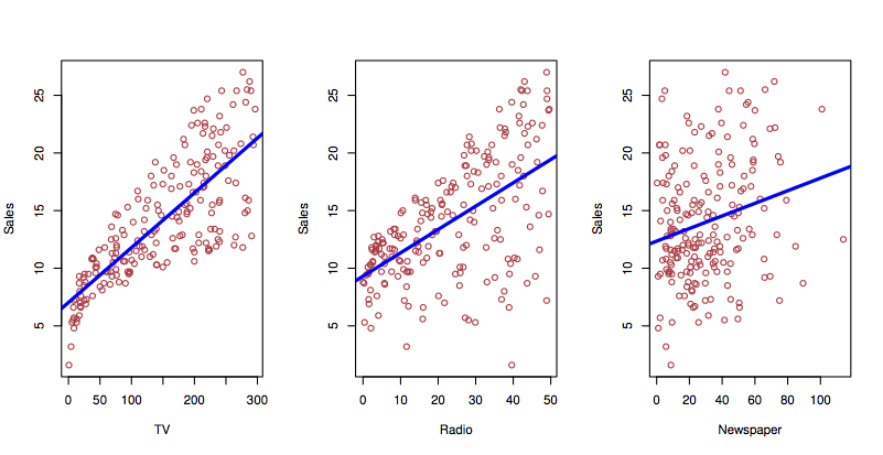
Perhaps effect of TV goes as sqrt(money) as media get saturated?
Perhaps there is a synergy that wasn’t included in the model?

2.11.1 Theory of whole-model ANOVA.

Standard measure: $\frac{\mbox{Explained amount}}{\mbox{Unexplained amount}}$

Examples:

Standard error of mean: $\frac{\hat{\mu}}{\sigma / n}$ – note the $n$.
t statistic on difference between two means: $\frac{\hat{\mu}_1 - \hat{\mu}_2}{\sigma / (n-1)}$
F statistic: $\frac{SS / df1}{SSR / df2}$
- df1 is the number of degrees of freedom involved by the model or model term under consideration.
- df2 is $n - (p - 1)$ where $p$ is the total degrees of freedom in the model. (I called this $m$ in the Math 155 book.) The intercept is what the $-1$ is about: the intercept can never account for case-to-case variation.

Trade-off between eating variance and consuming degrees of freedom.

2.12 Forward, backward and mixed selection

Use the College model to demonstrate each of the approaches by hand. Start with pairs() or write an lapply() for the correlation with Yield?

Create a whole bunch of model terms

“main” effects
“interaction” effects
nonlinear transformations: powers, logs, sqrt, steps, …
categorical variables

Result: a set of $k$ vectors that we’re interested to use in our model.

Considerations:

not all of the $k$ vectors may pull their weight
two or more vectors may overlap in how they eat up variance

Algorithmic approaches:

Try all combinations, pick the best one.
- computationally expensive/impossible $2^k$ possibilities
- what’s the sensitivity of the process to the choice of training data?
“Greedy” approaches

2.13 Programming Basics: Functions

Syntax of functions:

name <- function(arg1, arg2, ...) {
  body of function. Can use arg1, arg2, etc. 
}

typically you will return a value. The value calculated by the last command line in the body is what’s returned. Or you can use return() at any point in the function.
Often functions are designed to produce “side effects”, e.g. graphics.
Scope: what happens in functions stays in functions.

Create a plotting frame: plot()
- Write a function that makes this more convenient to use. What features would you like.
```
blank_frame <- function(xlim, ylim) {

}
```
Write a function to draw a circle.
- What do you want the interface to look like? What arguments are essential? What options are nice to have?

2.14 In-class programming activity

Histogram and density functions

set.seed(101)
n = 20
X <- data.frame(vals = runif(n), 
                group = as.character((1:n) %% 2))
ggplot(head(X, 6), aes(x = vals)) + 
  geom_density(bw = 1, position = "stack", aes(color = group, fill = group)) + 
  geom_rug(aes(color = group)) + 
 # facet_grid( . ~ group) +
  xlim(-0.5, 1.5)

Day 6 activity

2.15 Review of Day 7

We finished reviewing adjusted R^2 and ANOVA.
Started talking about linear algebra.

We only got through the first few elements in our review of linear algebra. Let’s go through them again

2.16 Using predict() to calculate precision

confidence intervals
prediction intervals

2.17 Conclusion

This wraps up our look at linear regression. Main points:

model output is a linear combination of the inputs.
lm() finds the “best” linear combination.
rich theory relating to precision of coefficients and the residuals.
traditional ways of applying that theory: F tests and t tests.