Topic 5 Linear and Quadratic Discriminant Analysis
5.1 Example: Default on student loans
model_of_default2 <-
  lda(default ~ balance + income, data = Default)
model_of_default2
## Call:
## lda(default ~ balance + income, data = Default)
##
## Prior probabilities of groups:
## No Yes
## 0.9667 0.0333
##
## Group means:
## balance income
## No 803.9438 33566.17
## Yes 1747.8217 32089.15
##
## Coefficients of linear discriminants:
## LD1
## balance 2.230835e-03
## income 7.793355e-06predict(model_of_default2, newdata = list(balance = 3000, income = 40000))## $class
## [1] Yes
## Levels: No Yes
##
## $posterior
## No Yes
## 1 0.008136798 0.9918632
##
## $x
## LD1
## 1 4.879445sector_mod <- lda(sector ~ wage + educ, data = CPS85)
sector_mod## Call:
## lda(sector ~ wage + educ, data = CPS85)
##
## Prior probabilities of groups:
## clerical const manag manuf other prof
## 0.18164794 0.03745318 0.10299625 0.12734082 0.12734082 0.19662921
## sales service
## 0.07116105 0.15543071
##
## Group means:
## wage educ
## clerical 7.422577 12.93814
## const 9.502000 11.15000
## manag 12.704000 14.58182
## manuf 8.036029 11.19118
## other 8.500588 11.82353
## prof 11.947429 15.63810
## sales 7.592632 13.21053
## service 6.537470 11.60241
##
## Coefficients of linear discriminants:
## LD1 LD2
## wage 0.06196785 -0.2108914
## educ 0.43349567 0.2480535
##
## Proportion of trace:
## LD1 LD2
## 0.9043 0.0957predict(sector_mod, newdata = list(wage = 10, educ = 16))## $class
## [1] prof
## Levels: clerical const manag manuf other prof sales service
##
## $posterior
## clerical const manag manuf other prof
## 1 0.1619905 0.005807399 0.1680084 0.02274195 0.04429026 0.4781032
## sales service
## 1 0.07668742 0.04237084
##
## $x
## LD1 LD2
## 1 1.352846 0.5336987all_combos <- expand.grid(wage = seq(0,20,length=100), educ = seq(5,16, length = 100))
res <- predict(sector_mod, newdata = all_combos)$class
all_combos$predicted <- res
ggplot(all_combos, aes(x = wage, y = educ, color = predicted)) + geom_point()
5.2 A Bayes’ Rule approach
Suppose we have \(K\) classes, \(A_1, A_2, \ldots, A_K\). We also have a set of inputs \(x_1, x_2, \ldots, x_p \equiv {\mathbf x}\).
We observe \({\mathbf x}\) and we want to know \(p(A_j \downarrow {\mathbf x})\). This is a posterior probability.
Per usual, the quantities we can get from our training data are in the form of a likelihood: \(p({\mathbf x} \downarrow A_j)\).
Given a prior \(p(A_j)\) for all K classes, we can flip the likelihood into a posterior.
In order to define our likelihood \(p({\mathbf x} \downarrow A_j)\), we need both the training data and a model form for the probability \(p()\).
A standard (but not necessarily good) model of a distribution is a multivariate Gaussian. LDA and QDA are based on a multi-variable Gaussian.
5.3 Univariate Gaussian
\[p(x) = \underbrace{\frac{1}{\sqrt{2 \pi \sigma^2}}}_{Normalization} \underbrace{\exp(- \frac{(x-m)^2}{2 \sigma^2})}_{Shape}\]
Imagine that we have another variable \(z = x/3\). Geometrically, \(z\) is a stretched out version of \(x\), stretched by a factor of 3 around the mean. The distribution is
\[p(z) = \underbrace{\frac{1}{\sqrt{2 \pi (3\sigma)^2}}}_{Normalization}\ \underbrace{\exp(- \frac{(x-m)^2}{2 (3\sigma)^2})}_{Shape}\]
Note how the normalization changes. \(p(z)\) is broader than \(p(x)\), so it must also be shorter.
The R function dnorm() calculates \(p(x)\) for a univariate Gaussian.
5.5 Bivariate normal distribution with correlations
\[f(x,y) = \frac{1}{2 \pi \sigma_X \sigma_Y \sqrt{1-\rho^2}} \exp\left( -\frac{1}{2(1-\rho^2)}\left[ \frac{(x-\mu_X)^2}{\sigma_X^2} + \frac{(y-\mu_Y)^2}{\sigma_Y^2} - \frac{2\rho(x-\mu_X)(y-\mu_Y)}{\sigma_X \sigma_Y} \right] \right)\]
If \(\rho > 0\) and \(x\) and \(y\) are both above their respective means, the correlation term makes the result less surprising: a larger probability.
Another way of writing this same formula is using a covariate matrix \({\boldsymbol\Sigma}\).
Or, in matrix form
\[(2\pi)^{-\frac{k}{2}}|\boldsymbol\Sigma|^{-\frac{1}{2}}\, \exp\left( -\frac{1}{2}(\mathbf{x}-\boldsymbol\mu)'\boldsymbol\Sigma^{-1}(\mathbf{x}-\boldsymbol\mu) \right)\]
where \[\boldsymbol \Sigma \equiv \left(\begin{array}{cc}\sigma_x^2 & \rho \sigma_x \sigma_y\\\rho\sigma_x\sigma_y& \sigma_y^2\end{array} \right)\]
Therefore \[\boldsymbol \Sigma^{-1} \equiv \frac{1}{\sigma_x^2 \sigma_y^2 (1 - \rho^2)} \left(\begin{array}{cc}\sigma_y^2 & - \rho \sigma_x \sigma_y\\ - \rho\sigma_x\sigma_y& \sigma_x^2\end{array} \right)\]
5.6 Shape of multivariate gaussian
As an amplitude plot 
Showing marginals and 3-\(\sigma\) contour 
5.7 Generating bivariate normal from independent
We want to find a matrix, M, by which to multiply iid Z to get correlated X with specified \(\sigma_x, \sigma_y, \rho\). The covariance matrix will be
# parameters
sigma_x <- 3
sigma_y <- 1
rho <- 0.5
Sigma <- matrix(c(sigma_x^2, rho * sigma_x * sigma_y, rho * sigma_x * sigma_y, sigma_y^2), nrow = 2)
n <- 5000 # number of simulated cases
# iid base
Z <- cbind(rnorm(n), rnorm(n))
M <- matrix(c(sigma_x, 0, rho * sigma_y, sqrt(1-rho^2)* sigma_y), nrow = 2)
X <- Z %*% M
cov(X)
## [,1] [,2]
## [1,] 8.667761 1.4328505
## [2,] 1.432851 0.9602763M transforms from iid to correlated.
In formula, we transform from correlated X to iid, so use M\(^{-1}\).
5.8 Independent variables \(x_i\)
- Describing dependence
x1 = runif(1000)
x2 = rnorm(1000, mean=3*x1+2, sd=x1)
plot(x1, x2)
- Linear correlations and the Gaussian
Remember the univariate Gaussian with parameters \(\mu\) and \(\sigma^2\):
\[\frac{1}{\sqrt{2 \pi \sigma^2}} \exp \left(-\frac{(x - \mu)^2}{2 \sigma^2}\right)\]
Situation: Build a classifier. We measure some features and want to say which group a case refers to.
Specific example: Based on the ISLR::Default data, find the probability of a person defaulting on a loan given their income and balance.
names(Default)## [1] "default" "student" "balance" "income"ggplot(Default,
aes(x = income, y = balance, alpha = default, color = default)) +
geom_point()
We were looking at the likelihood: prob(observation | class)
Note: Likelihood itself won’t do a very good job, since defaults are relatively uncommon. That is, p(default) \(\ll\) p(not).
5.9 Re-explaining \(\boldsymbol\Sigma\)
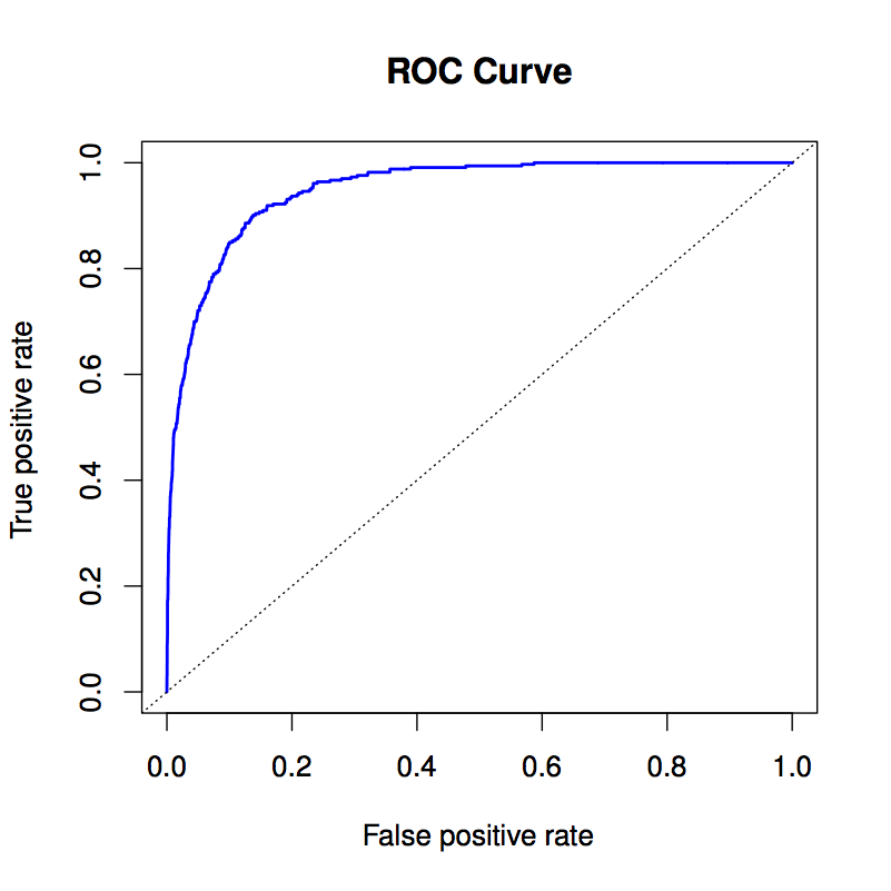
Figure 5.1: Figure 4.8 from ISL
Imagine two zero-mean variables, \(x_i\) and \(x_j\), e.g. education and age, and suppose that \(v_i = x_i - \mu_i\) and \(v_j = x_j - \mu_j\). I’ll write these in data table format, where each column is a variable and each row is a case and denote this by
\(\left(\begin{array}{c}v_i\\\downarrow\end{array}\right)\) and \(\left(\begin{array}{c}v_j\\\downarrow\end{array}\right)\)
Correlations between random variables \((v_i, v_j)\) are created by overlapping sums of zero-mean iid random variables \((z_i, z_j)\),
\[\left(\begin{array}{cc}v_i &v_j\\\downarrow & \downarrow\end{array}\right) = \left(\begin{array}{cc}z_i & z_j \\ \downarrow & \downarrow\end{array}\right) \left(\begin{array}{cc}a & b\\0 & c\end{array}\right) \equiv \left(\begin{array}{cc}z_i & z_j\\\downarrow & \downarrow\end{array}\right) {\mathbf A} \]
and add in a possibly non-zero mean to form each \(x\). \[\left(\begin{array}{cc}x_i &x_j\\\downarrow&\downarrow\end{array}\right) = \left(\begin{array}{cc}v_i & v_j\\\downarrow&\downarrow\end{array}\right) + \left(\begin{array}{cc}m_i & m_j\\\downarrow&\downarrow\end{array}\right) \] where each of \(\left(\begin{array}{c}m_i\\|\end{array}\right)\) and \(\left(\begin{array}{c}m_i\\|\end{array}\right)\) have every row the same.
The covariance matrix \(\boldsymbol\Sigma\) is
\[{\boldsymbol \Sigma} \equiv \frac{1}{n} \left(\begin{array}{cc}v_i & v_j\\\downarrow&\downarrow\end{array}\right)^T \left(\begin{array}{cc}v_i & v_j\\\downarrow&\downarrow\end{array}\right) = \frac{1}{n} \left(\begin{array}{c}v_i \longrightarrow\\v_j \longrightarrow\end{array}\right) \left(\begin{array}{cc}v_i & v_j\\\downarrow&\downarrow\end{array}\right) \]
Substituting in
\[ \left(\begin{array}{cc}v_i &v_j\\\downarrow & \downarrow\end{array}\right) = \left(\begin{array}{cc}z_i & z_j\\\downarrow & \downarrow\end{array}\right) {\mathbf A} \] we get
\[{\boldsymbol \Sigma} = \frac{1}{n} \left[\left(\begin{array}{cc}z_i & z_j\\\downarrow & \downarrow\end{array}\right) {\mathbf A} \right]^T \left(\begin{array}{cc}z_i & z_j\\\downarrow & \downarrow\end{array}\right) {\mathbf A} = \frac{1}{n} {\mathbf A}^T \left(\begin{array}{c}z_i \longrightarrow\\z_j \longrightarrow\end{array}\right) \left(\begin{array}{cc}z_i & z_j\\\downarrow & \downarrow\end{array}\right) {\mathbf A}\]
Now \(\left(\begin{array}{cc}z_i & z_j\\\downarrow & \downarrow\end{array}\right)\) are iid with zero mean and unit variance, so \[\left(\begin{array}{c}z_i \longrightarrow\\z_j \longrightarrow\end{array}\right) \left(\begin{array}{cc}z_i & z_j\\\downarrow & \downarrow\end{array}\right) = \left(\begin{array}{cc}1 & 0\\0 & 1\end{array}\right)\] so \({\boldsymbol \Sigma} = {\boldsymbol A}^T {\boldsymbol A}\).
In other words, \(\boldsymbol A\) is the Choleski decomposition of \(\boldsymbol \Sigma\).
Operationalizing this in R
- Find \(\boldsymbol \Sigma\) from data:
cov(data), e.g.
library(dplyr)
Sigma <- cov(ISLR::Default %>% dplyr::select(balance, income))
Sigma
## balance income
## balance 233980.2 -982142.3
## income -982142.3 177865954.8- Find \(\boldsymbol A\) from \(\boldsymbol \Sigma\)
A <- chol(Sigma)
A
## balance income
## balance 483.715 -2030.415
## income 0.000 13181.175- Generate iid \(\left(\begin{array}{cc}z_i&z_j\\\downarrow&\downarrow\end{array}\right)\) with unit variance
n <- 100 # say
Z <- cbind(rnorm(n), rnorm(n))- Create the correlated \(\left(\begin{array}{cc}v_i&v_j\\\downarrow&\downarrow\end{array}\right)\) from \(\left(\begin{array}{cc}z_i&z_j\\\downarrow&\downarrow\end{array}\right)\)
V <- Z %*% A- Create a set of means \(\left(\begin{array}{cc}m_i&m_j\\\downarrow&\downarrow\end{array}\right)\) to add on to \(\left(\begin{array}{cc}v_i&v_j\\\downarrow&\downarrow\end{array}\right)\)
M <- cbind(rep(3, n), rep(-2, n))
head(M)
## [,1] [,2]
## [1,] 3 -2
## [2,] 3 -2
## [3,] 3 -2
## [4,] 3 -2
## [5,] 3 -2
## [6,] 3 -2- Add \(\left(\begin{array}{cc}m_i&m_j\\\downarrow&\downarrow\end{array}\right)\) to \(\left(\begin{array}{cc}v_i&v_j\\\downarrow&\downarrow\end{array}\right)\) to create \(\left(\begin{array}{cc}x_i&x_j\\\downarrow&\downarrow\end{array}\right)\)
X <- V + M- Find the covariance matrix for \(\left(\begin{array}{cc}x_i&x_j\\\downarrow&\downarrow\end{array}\right)\)
cov(X)## balance income
## balance 208366.0 -861153.5
## income -861153.5 160224764.8Why isn’t this exactly the same as the covariance matrix \(\boldsymbol \Sigma\) that we were aiming at? Because of random fluctuations in the \(\left(\begin{array}{cc}z_i&z_j\\\downarrow&\downarrow\end{array}\right)\). You can reduce the impact of those fluctuations by making \(n\) bigger.
Notice that \({\boldsymbol A}\) transforms from uncorrelated \(\left(\begin{array}{cc}z_i&z_j\\\downarrow&\downarrow\end{array}\right)\) to correlated \(\left(\begin{array}{cc}v_i&v_j\\\downarrow&\downarrow\end{array}\right)\). If we have \(\left(\begin{array}{cc}x_i&x_j\\\downarrow&\downarrow\end{array}\right)\), we can create the uncorrelated \(\left(\begin{array}{cc}z_i&z_j\\\downarrow&\downarrow\end{array}\right)\) with \[\left(\begin{array}{cc}z_i&z_j\\\downarrow&\downarrow\end{array}\right) = \left[\left(\begin{array}{cc}x_i&x_j\\\downarrow&\downarrow\end{array}\right) - \left(\begin{array}{cc}m_i&m_j\\\downarrow&\downarrow\end{array}\right)\right] {\boldsymbol A}^{-1}\].
Recall \[(2\pi)^{-\frac{k}{2}}|\boldsymbol\Sigma|^{-\frac{1}{2}}\, \exp\left( -\frac{1}{2}(\mathbf{x}-\boldsymbol\mu)^T\boldsymbol\Sigma^{-1}(\mathbf{x}-\boldsymbol\mu) \right)\].
Since \(\boldsymbol\Sigma = \boldsymbol A^T \boldsymbol A\) and \(x_i - m = v_i\), this formula is equivalent to \[(2\pi)^{-\frac{k}{2}}|\boldsymbol\Sigma|^{-\frac{1}{2}}\, \exp\left( -\frac{1}{2}(\mathbf{v}^{T}\boldsymbol A^{-T} \boldsymbol A^{-1} \mathbf v) \right) = (2\pi)^{-\frac{k}{2}}|\boldsymbol\Sigma|^{-\frac{1}{2}}\, \exp\left( -\frac{1}{2}(\mathbf{z}^{T}\mathbf z) \right)\] Now for a pair of values like \(\mathbf x = (x_1 \ \ x_2)\) finding the probability of \(\mathbf x\) corresponds to finding the corresponding \(\mathbf z^T = (z_i\ \ z_j)\), where \(z_i\) and \(z_j\) are each a random scalars, and \((\mathbf{z}^{T}\mathbf z) = z_i^2 + z_2^2\), so the probability is
\[(2\pi)^{-\frac{k}{2}}|\boldsymbol\Sigma|^{-\frac{1}{2}}\, \exp\left( -\frac{1}{2}(z_1^2 + z_2^2 )\right) = (2\pi)^{-\frac{k}{2}}|\boldsymbol\Sigma|^{-\frac{1}{2}}\, \exp(-\frac{z_1^2}{2}) \exp(-\frac{z_2^2}{2})\]
Look at the stretching that goes on due to a matrix:
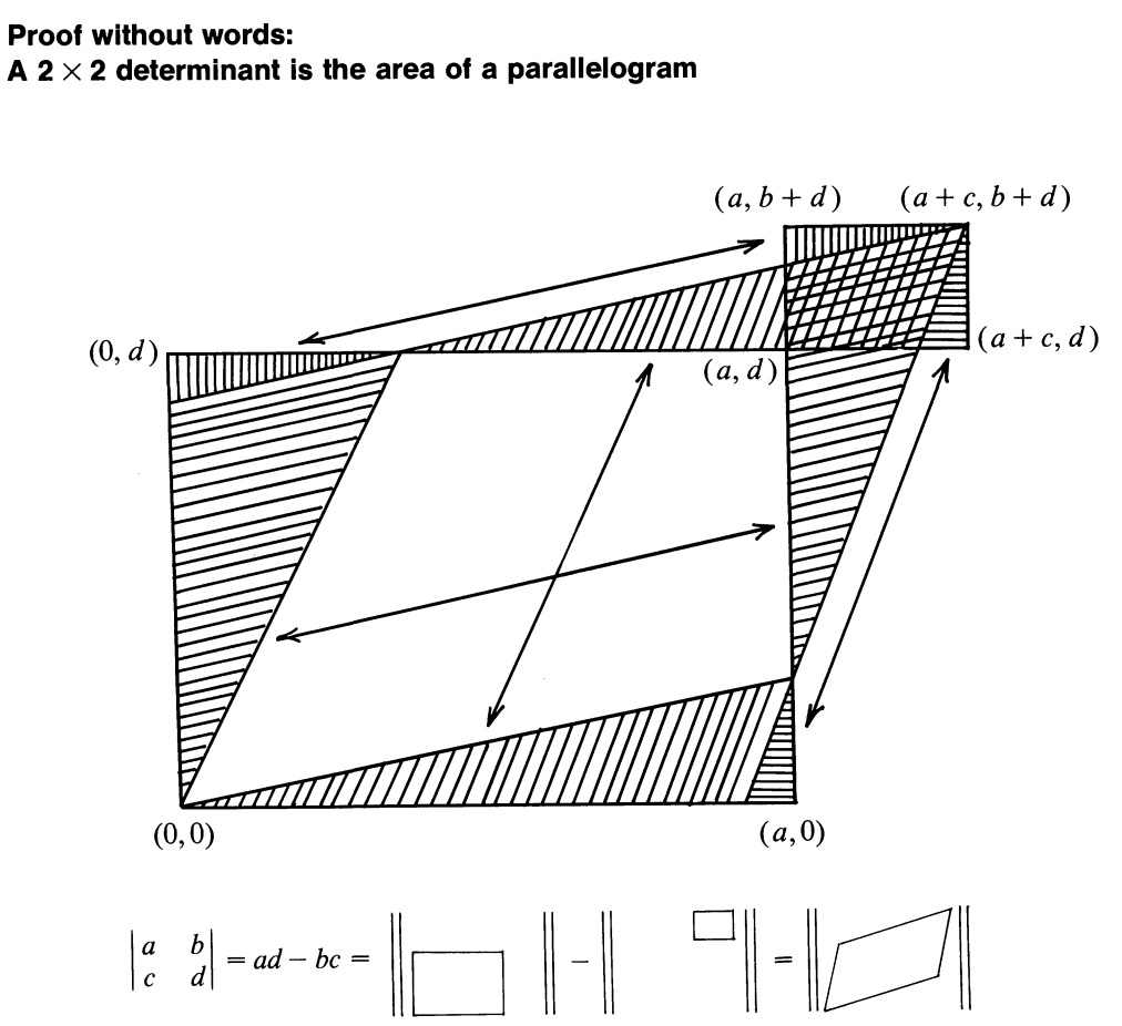
The stretching is due to the matrix \(\boldsymbol A\). So we should divide by the determinant of \(\boldsymbol A\), that is, \(|\boldsymbol A|\). The nature of the Cholesky decomposition is that \(|\boldsymbol A| = \sqrt{|\boldsymbol\Sigma|}\). Note in the formula for the Gaussian that the normalizing constant involves \(\sqrt{|\boldsymbol\Sigma|}\).
5.10 LDA
All classes are treated as having the same \({\mathbf \Sigma}\).
5.11 QDA
Classes are treated with different \({\mathbf \Sigma}_i\).
knitr::include_graphics("Images/Chapter-4/4.9.png")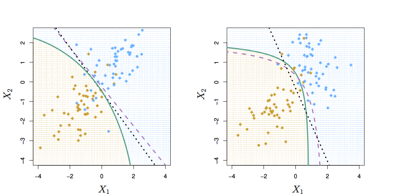
Figure 5.2: Figure 4.9 from ISL. Left: Bayes (purple dashed), LDA (black dotted), and QDA (green solid)} decision boundaries for a two-class problem with \({\mathbf \Sigma}_1 = {\mathbf \Sigma}_2\). Right: QDA
5.12 Error test rates on various classifiers
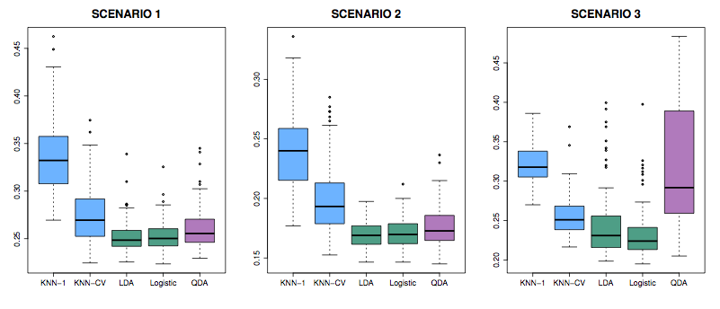
Figure 5.3: Figure 4.10 from ISL
Scenarios: In all, class means are different.
- Each class is two uncorrelated Gaussian random vars.
- Both classes had a correlation of \(-0.5\)
- Uncorrelated, like (1), but the distribution is t(df=?): long tailed to right.
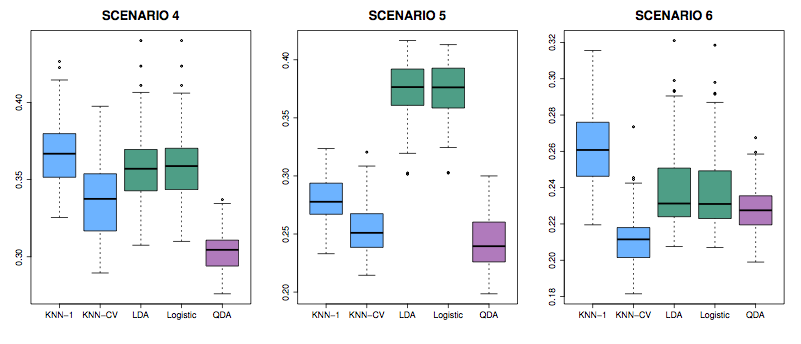
Figure 5.4: Figure 4.11 from ISL
- Like (2), but one class has \(\rho = 0.5\) and the other \(\rho = -0.5\)
- A nonlinear predictor with \(X_1^2\), \(X_2^2\), \(X_1 \times X_2\) giving a quadratic decision boundary
- A decision boundary more complicated than a quadratic.
5.13 Error rates
Ways to measure the performance of a classifier.
Examples: Two classifiers of employment type.
data(CPS85, package = "mosaicData")
classifier_1 <- lda(sector ~ wage + educ + age, data = CPS85)
classifier_2 <- qda(sector ~ wage + educ + age, data = CPS85)- Confusion matrix
table(CPS85$sector, predict(classifier_1)$class)##
## clerical const manag manuf other prof sales service
## clerical 60 0 0 1 17 17 0 2
## const 7 0 2 4 5 0 0 2
## manag 15 0 5 1 3 31 0 0
## manuf 22 0 4 13 14 7 0 8
## other 21 0 2 6 24 5 0 10
## prof 15 0 2 0 6 81 0 1
## sales 25 0 1 0 2 8 0 2
## service 38 0 1 9 12 7 0 16- Rates for right-vs-wrong.
- Accuracy. Total error rate. Not generally useful, because there are two ways to be wrong.
table(predict(classifier_1)$class == CPS85$sector) / nrow(CPS85)## ## FALSE TRUE ## 0.6273408 0.3726592- Sensitivity: If the real class is X, the probability that the classifier will produce an output of X. We need to choose the output we care about. Let’s use
prof.
is_prof <- CPS85$sector == "prof"
predicts_prof <- predict(classifier_1)$class == "prof"
table(is_prof, predicts_prof)
105 actual## predicts_prof ## is_prof FALSE TRUE ## FALSE 354 75 ## TRUE 24 81prof, of which 81 were correctly classified. So, sensitivity is 81/105.- Specificity: If the real class is not X, the probability that the classifier will output not X. See above table. 429 not
prof, of which 354 were correctly classified. So specificity is 354/429.
- Loss functions
- Social awkwardness of thinking someone is in the wrong profession.
5.14 Receiver operating curves
There’s always one or more parameters that can be set in a classifier. This might be as simple as the prior probability.
As this parameter is changed, typically sensitivity will go up at the cost of specificity, or vice versa.
President Garfield’s assassination.