Topic 6 Cross-Validation and Bootstrapping
In making a statistical model (including with machine-learning techniques) we have an overall goal:
Make model error small for the ways the model will actually be applied.
Model error has three components:
- irreducible error (\(\epsilon\))
- error due to bias
- error due to variance
Bias refers to the ways that \(\hat{f}({\mathbf X})\) is systematically different from the idealized \(f({\mathbf X})\).
Variance refers to the ways that \(\hat{f}_i({\mathbf X})\) varies with the particular sample \(i\) used for training.
The overall model error is the sum of squares of these three components.
There’s nothing to be done about irreducible error.
we want to do two things that can conflict with one another:
- make bias small.
- flexible models
- QDA rather than LDA
- include lots of explanatory variables
- make variance small
- lots of data
- few degrees of freedom (vs. flexibility or QDA)
- avoid collinearity and weak/irrelevant explanatory variables
6.1 Philosophical approaches
Often, these are just drawing attention to the problem; they don’t actually offer a solution.
6.1.1 Occam’s Razor: A heuristic
Non sunt multiplicanda entia sine necessitate.
- Entities must not be multiplied beyond necessity.
But what’s “beyond necessity?”
6.1.2 Einstein’s proverb
Man muß die Dinge so einfach wie möglich machen. Aber nicht einfacher.
- Make things as simple as possible, but not one bit simpler.
But what’s “too simple?”
Basic modeling-building question:
- Does adding this [variable, model term, potential flexibility] help?
- For reducing bias: yes
- For reducing variance: maybe (if it eats up residual variance)
- For reducing error: maybe
6.2 Operationalizing model choice
We need to be able to measure two aspects of a model:
- bias: theory is difficult, since we don’t know the “true” system
- variance: theory is straightforward
Bias in practice:
- Have a good measure of variance.
- Add in new model terms, flexibility, etc. See if the variance goes down.
Think in terms of comparing two models to select which one is better.
“Better” needs to be transitive: if A is better than B, and B is better than C, then A is better than C.
Then, any number of models can be compared to find the one (or more) that is the best.
6.3 Some definitions of “better”
- Larger likelihood (non-iid Gaussian error models)
- Smaller mean square prediction error (same as larger likelihood with iid Gaussian error model)
- Classification error rate is smaller
- Loss function is smaller
6.4 Training and Testing
Evaluation of performance using training data is biased to give larger likelihood (smaller MSE or classification error or loss error).
Unbiased evaluation is done on separate testing data.
6.5 Trade-off
Need large testing dataset for good estimate of performance
Need large training dataset for reducing variance in fit.
How to get both:
- Collect a huge amount of data. When this works, go for it!
- K-fold cross validation
- Pull out 1/K part of the data for performance testing.
- Fit to the other (K-1)/K part of the data.
- Repeat K times and average the prediction results over the K trials.
- Once you’ve found the best form of model, fit it to the whole data set. That’s your model.
6.6 Classical theory interlude
M-estimators and robust estimation.
6.7 Bootstrapping
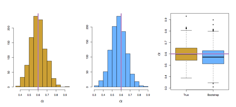
Figure 6.1: ISLR Figure 5.10
In-class demonstration.
- How many cases don’t get used in a typical resample?
- Hint: It will suffice to work with indices, so the numbers
1:nfor a sample of sizen.
cases <- 1:10000
ntrials <- 50
result <- numeric(ntrials)
for (k in 1:50) {
  bootstrap_sample <- sample(cases, size=length(cases), replace = TRUE)
  result[k] <- length(setdiff(cases, unique(bootstrap_sample))) / length(cases)
}
result
## [1] 0.3647 0.3686 0.3633 0.3693 0.3661 0.3742 0.3680 0.3651 0.3671 0.3696
## [11] 0.3671 0.3687 0.3663 0.3719 0.3678 0.3622 0.3744 0.3691 0.3703 0.3678
## [21] 0.3677 0.3673 0.3639 0.3677 0.3685 0.3664 0.3709 0.3695 0.3688 0.3680
## [31] 0.3638 0.3665 0.3714 0.3735 0.3638 0.3656 0.3676 0.3688 0.3783 0.3663
## [41] 0.3678 0.3628 0.3731 0.3735 0.3741 0.3729 0.3592 0.3732 0.3662 0.3679## Or ...
(1 - 1/length(cases))^length(cases)## [1] 0.367861library(mosaic)
do(100) * {
n <- 100000
s <- sample(1:n, size = n, replace = TRUE)
n - length(unique(s))
}## result
## 1 36798
## 2 36631
## 3 36705
## 4 36724
## 5 36846
## 6 36784
## 7 36725
## 8 36742
## 9 36825
## 10 36768
## 11 36646
## 12 36839
## 13 36965
## 14 36608
## 15 36789
## 16 36748
## 17 36728
## 18 36849
## 19 36640
## 20 36888
## 21 36846
## 22 36882
## 23 36794
## 24 36731
## 25 36875
## 26 36754
## 27 36793
## 28 36720
## 29 36556
## 30 36679
## 31 36787
## 32 36801
## 33 36644
## 34 36852
## 35 36713
## 36 36649
## 37 36707
## 38 36615
## 39 36753
## 40 36555
## 41 36776
## 42 36900
## 43 36829
## 44 36977
## 45 36787
## 46 36610
## 47 36952
## 48 36853
## 49 36698
## 50 36927
## 51 37008
## 52 36688
## 53 36734
## 54 36848
## 55 36780
## 56 36872
## 57 36796
## 58 36785
## 59 36680
## 60 36813
## 61 36646
## 62 36816
## 63 36696
## 64 36813
## 65 36904
## 66 36689
## 67 36690
## 68 36760
## 69 36807
## 70 36748
## 71 36672
## 72 36866
## 73 36801
## 74 36760
## 75 36672
## 76 36767
## 77 36945
## 78 36713
## 79 36765
## 80 36584
## 81 36802
## 82 36912
## 83 36711
## 84 36876
## 85 36682
## 86 36704
## 87 36824
## 88 36728
## 89 36752
## 90 36844
## 91 36740
## 92 36816
## 93 36797
## 94 36823
## 95 36975
## 96 36734
## 97 36845
## 98 36694
## 99 36771
## 100 36714