# calculating the LR
3.89 / 0.456
[1] 8.530702A real-world experiment is underway right now involving millions of people in a life-or-death situation. Or, perhaps that is too dramatic. The experiment we have in mind concerns the testing of self-driving taxis in urban areas. Companies like Waymo have deployed fleets of self-driving cars that offer a taxi service.
How safe are these cars? That the testing is being allowed at all says something. How much experience will we need with the cars to be sure that we are making a proper judgment?
As of this writing, companies have been running pilot programs deploying self-driving taxis in a handful of cities. They have already collected substantial amounts of data and reported summaries such as this Waymo bulletin. Rather than comment on this data, we will imagine ourselves at a hypothetical time when we had only vague prior beliefs or opinions about the safety of the self-driving cars. Then, we will gradually accumulate (made-up) data to see how applying Bayesian methods enables us to update and refine our beliefs. We will keep it realistic, but because it is made-up, do not use this example to draw conclusions about the real world.
“Safety” is a variable. To represent it quantitatively, we need to operationalize it: translate it into a quantity that can be recorded for each car. Our operationalization in this demonstration will be the number of miles driven by each car from the time it enters service until the first accident. Alternatively, for those cars that have not yet had an accident, the number of miles driven up to the point at which we analyze the data. A car that goes a large number of miles without an accident provides evidence that the fleet has high safety. A car that has an accident after a small number of miles is a counter-indication; evidence that the fleet safety is poor. To determine fleet safety, we need to compile the evidence generated by each car in the fleet.
There are two kinds of uncertainty involved here. One: uncertainty about the fleet’s safety. However, even if we knew for sure the precise level of fleet safety, a second form of uncertainty remains: whether and when a given car will be in an accident.
Let us start with the second form of uncertainty, the one that pertains to individual cars. We would represent this uncertainty (as described in Chapter 7) with a probability distribution. An appropriate family of distributions to use is the exponential family. Exponential distributions model the time (or mileage, in our case) between incidents, as in the time from the start of the experiment until an accident. The rate parameter (\(\lambda\)) for the exponential distribution gives a concise quantitative measure of fleet safety. Our quantitative description of the uncertainty in fleet safety is a probability distribution on the \(\lambda\) parameter.
Historical data on human-driven cars suggests a rate of about five serious accidents per million vehicle miles. The quantity “five per million miles” is already in the proper form for \(\lambda\).
Suppose, for the sake of illustration, that there are two people involved in a debate about safety. One of them believes that self-driving cars are safer than human-driven cars. Call this person the enthusiast. Pressed for details, the enthusiast can express their opinion by claiming that the \(\lambda\) for the self-driving fleet is one accident per million miles. That is much safer than the historical record for human-driven cars suggests. The other person is a skeptic about the new technology. The skeptic insists that the accident rate is 10 accidents per million miles: twice the historical rate for human-driven cars. There are, of course, many other possible hypotheses, for instance, 4.3 accidents per million miles. However, for now, we will limit the competition to be between the enthusiast (1 per megamile) and the skeptic (10 per megamile).
The experiment starts. After about a year, we have collected some data (Table 10. 1) and calculated the likelihood of the data under each hypothesis to score the competition.
| car \(i\) | Status | Mileage |
|---|---|---|
| 1 | on road | 85,300 |
| 2 | on road | 65,200 |
| 3 | accident | 13,495 |
| 4 | on road | 131,200 |
| 5 | on road | 96,000 |
| 6 | accident | 54,682 |
| 7 | accident | 105,200 |
| 8 | on road | 53,900 |
| 9 | accident | 86,000 |
| 10 | on road | 94,300 |
The first two cars in the fleet have accumulated 85,300 and 65,200 without accident. The third car was in an accident at 13,495 miles.
Let us first focus on the evidence from the cars involved in an accident. Fig 10. 1 shows the probability distribution for the mileage until an accident, separately for the skeptic and the enthusiast. Note that under the enthusiast’s hypothesis, it is unlikely for a car to have an accident in, say, the first 100,000 miles. For the skeptic, on the other hand, such an accident is quite likely.
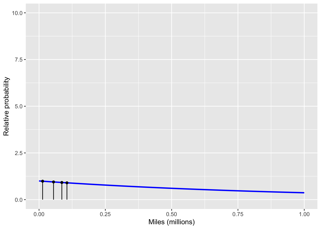
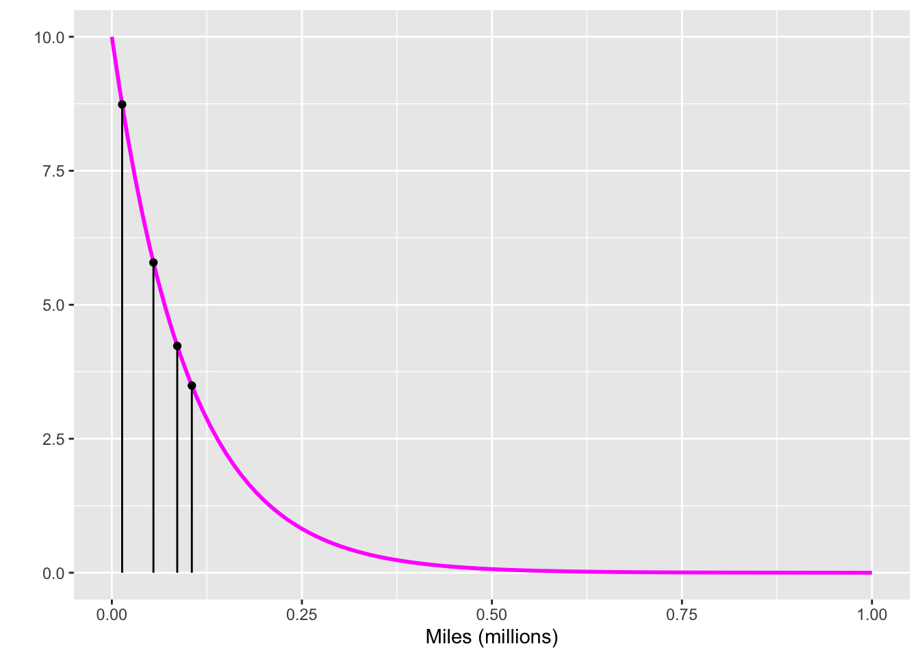
To calculate the likelihood of the data, under each hypothesis, multiply together the lengths of the black lines. For the enthusiast’s hypothesis, this comes to about 0.8. For the skeptic, about 750.0. Translating into a likelihood ratio, as described in Chapter 9, gives \(750 / 0.8 \approx 1000\). On the verbal scale given in Table 9.1, the likelihood ratio 1000 corresponds to “moderately strong” evidence. Win for the skeptic!
Actually, it is too early to declare a win. The game is only at halftime. Notice that there are ten cars in Table 10. 1. We have looked only at the four who had an accident. The other six also have something to say about safety.
For cars that had an accident, the exponential distribution family was appropriate; the accident data are already in the form needed to apply the probability distributions for the enthusiast and for the skeptic.
For cars that have not (yet) had an accident, we cannot use the exponential distribution in the likelihood calculation. To handle the data from non-accident cars, we need a probability distribution describing the mileage without an accident. We will show how to calculate this distribution in Chapter 13; we do not yet have the mathematical method needed. In the meantime, we show the appropriate distribution without justification.
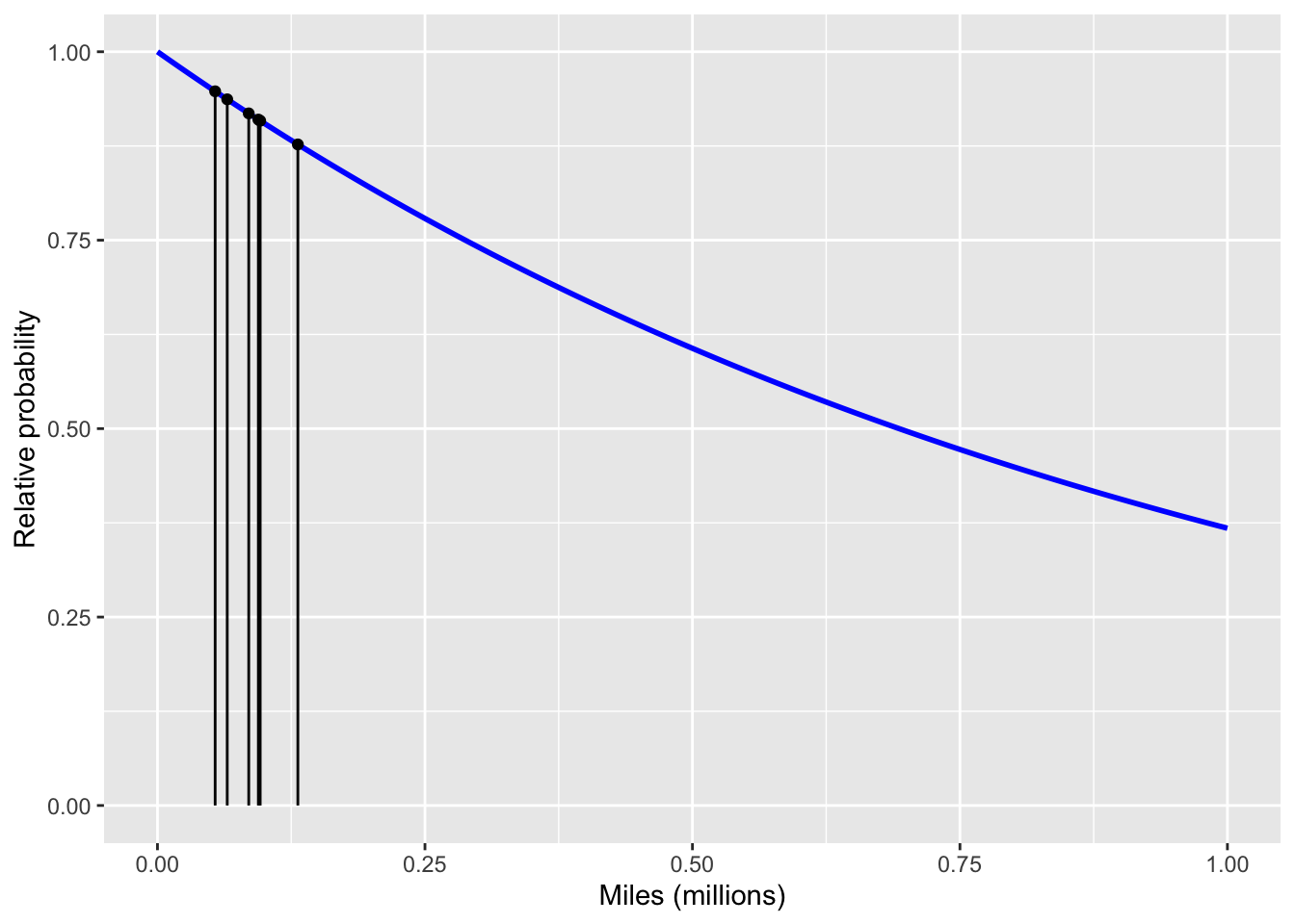
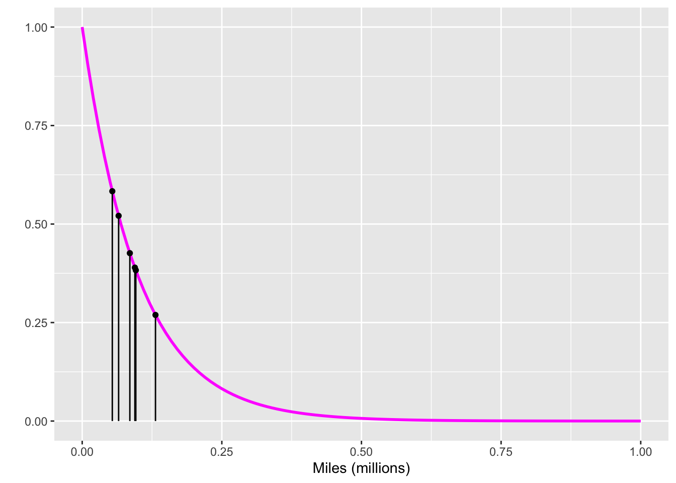
Figures 1 and 2 show the likelihood for all 10 of the cars under the different hypotheses held by the two advocates. For each advocate, we combine the evidence from the individual cars into an overall likelihood. As in Chapter 9, we accomplish this combination for each advocate, one at a time, simply by multiplying together the 10 individual likelihoods. The results in the competition between the skeptic and the enthusiast:
The skeptic is still vindicated, but not by so large a margin as when only the accident cars were considered. The ☞ likelihood ratio ☜ of skeptic to enthusiast is 8.5.
# calculating the LR
3.89 / 0.456[1] 8.530702On the verbal scale of evidence1, this is only “limited evidence” in favor of the more likely hypothesis.
In debate, a “straw man” argument sets up an opposing, weak proposition that is easy to refute. The enthusiastic advocate’s numerical claim prior to the experiment was that the accident rate was about 1 per million miles. Might this be a straw man? If so, the skeptic’s prior hypothesis (accident rate of 10 per million miles) will look good only by comparison to a weak opposing hypothesis.
We can avoid deception by a straw-man hypothesis by a relatively simple calculation. Rather than calculate the likelihood for just two hypotheses, consider many hypotheses in the competition covering a wide range of the parameter (accidents per million miles).
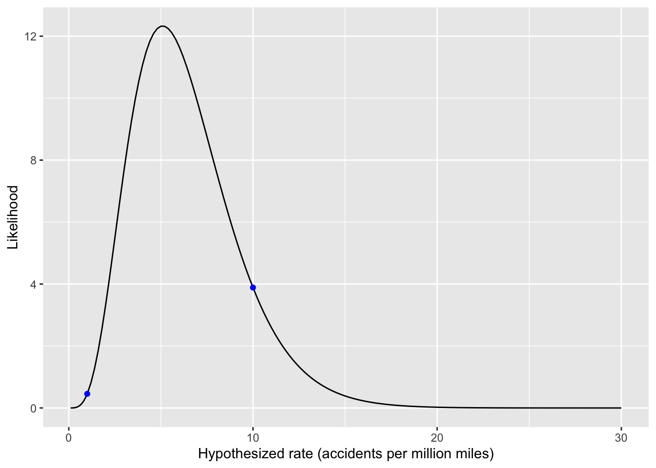
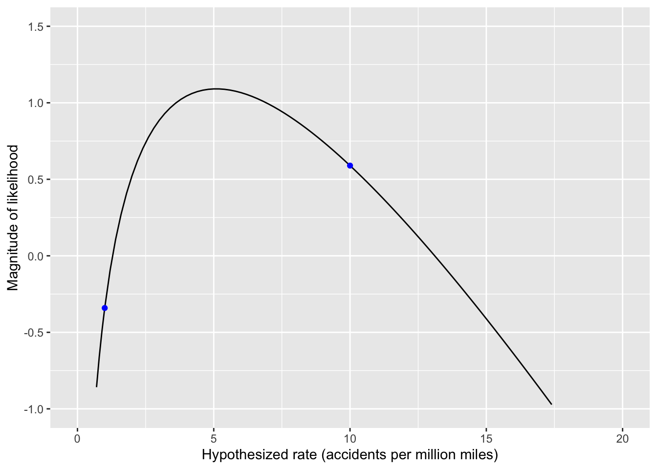
In the context of all possible hypothesized accident rates, the enthusiast’s hypothesis of one accident per million miles is looking a bit like a straw man. True, the skeptic’s hypothesis is better than the enthusiast’s. However, the skeptic’s hypothesis does not beat the hypothesis with the highest likelihood, which is five accidents per million miles.
The likelihood function does more than point to the most likely parameter. It tells us how uncertain we are about the parameter when confronted by the data.
The introduction to Chapter 7 described a very common way of expressing uncertainty, the \(\pm\) format so often found in scientific work. Statisticians call this a “confidence interval.” We can read off the confidence interval pretty directly from the graph of the likelihood function. For this purpose we look at the magnitude of the likelihood, shown in Fig 10. 3(b). To see how it works, recall the verbal scale for the strength of evidence in Table 9.1. There, a difference of 2 in magnitude between two hypotheses is considered “moderate evidence” for the more likely hypothesis. To construct the uncertainty interval, start with the magnitude likelihood for the most likely hypothesis: about five accidents per million miles. Then walk left along the curve. The likelihood, naturally, decreases because we started at the peak. Locate the hypothesis at which the magnitude likelihood is down to half of the peak, less than one accident per million miles in Fig 10. 3(b). That is the lower end of the uncertainty interval. Now return to the peak and walk to the right. Find where the magnitude likelihood is again at half the height of the peak; about 17 accidents per million miles in Fig 10. 3(b). Thus, the uncertainty interval is (roughly) 1 to 17 accidents per million miles.
That [1 to 17] uncertainty interval seems awfully broad to guide any real-world decision about whether self-driving cars are safe enough for regular use. That can be a valuable and important thing to know. It means that we do not have enough data (yet) to guide the decision.
To have doubted one’s own first principles is the mark of a civilized man. — Supreme Court Justice, Oliver Wendell Holmes, Jr (1841-1935)
Doubt is an uncomfortable condition, but certainty is a ridiculous one. — Voltaire (1694-1778)
The whole problem with the world is that fools and fanatics are always so certain of themselves, and wiser people so full of doubts. — Bertrand Russell (1872-1970)
Naturally, the enthusiast and the skeptic are each motivated to point to the role of chance in pushing the data away from their respective hypotheses.
We never mentioned how the enthusiast and the skeptic arrived at their hypotheses. It may be pure advocacy, for or against self-driving cars. If so, then each advocate can quantify the “truth” of their respective hypotheses by looking them up on the likelihood function.
Think about the phrase used in the previous paragraph: “Quantify the truth.” Common sense says that a proposition is either true or false; it cannot be in between. However, that in-betweenness is exactly what quantification points to. An expert quantitative reasoner will, for understandable reasons, use terms like “true” or “false” in everyday conversations. However, when it comes to hypotheses and data, those sharp distinctions do not apply, especially when there is little data.
The Bayesian framework replaces the true/false dichotomy with a genuine expression of uncertainty. As we have been doing since Chapter 7, we can express uncertainty as a probability distribution.
For the Bayesian, the likelihood function is only part of the story, albeit an essential part. The other part of the story is the uncertainty before the data were collected. This uncertainty is also expressed by a probability distribution, which in the Bayesian framework is called the ☞ prior ☜, a synonym for “before.” The Bayesian calculation is computationally simple: use the data to find the likelihood function, then multiply it by the prior. That product is yet another probability distribution, called the ☞ posterior ☜, as in “after the data have been incorporated into our thinking.”
In this sense, the prior is ☞ subjective ☜: different people can reasonably have different priors. This subjectivity is what led the Frequentists to deny the applicability of the Bayesian method. They have a point, since the priors held by the skeptic and enthusiast might have been pig-headedly narrow.
Imagine this conversation with the skeptic, but which might apply to the enthusiast as well.
You: “What’s your prior?”
Skeptic: “That the accident rate is 10 per million miles?”
You: “That’s not a probability distribution.”
Skeptic: “Yes, it is. My prior assigns probability 1 to the 10-per-million-miles rate, and zero to anything else.”
With such a prior, the posterior is pre-determined: it must be the same as the prior. That is, the skeptic’s subjective opinion entirely determines the result.
The Frequentists are right to be concerned about pig-headedness, but responsible people soften things a bit: “the accident rate is about 10 per million miles.” Now we have to define “about.”
For the Frequentist, who holds that parameters have a real existence and a precise value (that is not yet known), any amount of subjectivity gets in the way of the search for truth. A modeler’s point of view is different: a parameter is a quantity that’s part of a model. The parameter is real only because someone or a group of people used it to frame their model. Another model might not have that parameter. The modeler sees the Frequentist attitude as a reification of parameters.
We now return to the definition of a model: “A representation for a purpose.” Often, the purpose is to guide a decision. Moreover, decisions are often the result of debate among participants with differing views.
Supreme Court Justice Ruth Bader Ginsburg had a helpful view about debate. She said, “Fight for the things that you care about, but do it in a way that will lead others to join you.” One way to lead others to join you is to acknowledge the possibility that they might be right. In the Bayesian framework, this means broadening your prior to support the views of all (reasonable) people engaged in the debate. You do not have to assign much probability to those views, but you must assign some.
To give an example that has come up in debate about defenses against intercontinental ballistic missiles (ICBM), an article in The Atlantic2 reported that an office in the Pentagon claims that anti-ballistic missiles “have displayed a 100% accuracy rate in testing for more than a decade.” This statement was offered in response to a well-founded claim in the popular movie “House of Dynamite” that the accuracy rate is about 60%. The Pentagon based its claim on the results of the last four tests, only two of which involved an actual ICBM. The movie’s claim considered all 20 tests conducted since 1999.
Who is right? In the Bayesian framework, we do not demand right-or-wrong answers. Instead, we frame a prior, compute the likelihood function from the new data, and multiply the prior by the likelihood function to obtain the posterior.
We can form a prior based on the 16 tests that preceded the four most recent tests. Seven of those 16 tests were successful, a success rate of about 44%. Thus, a sensible prior for interpreting the last four tests should center on 44%.
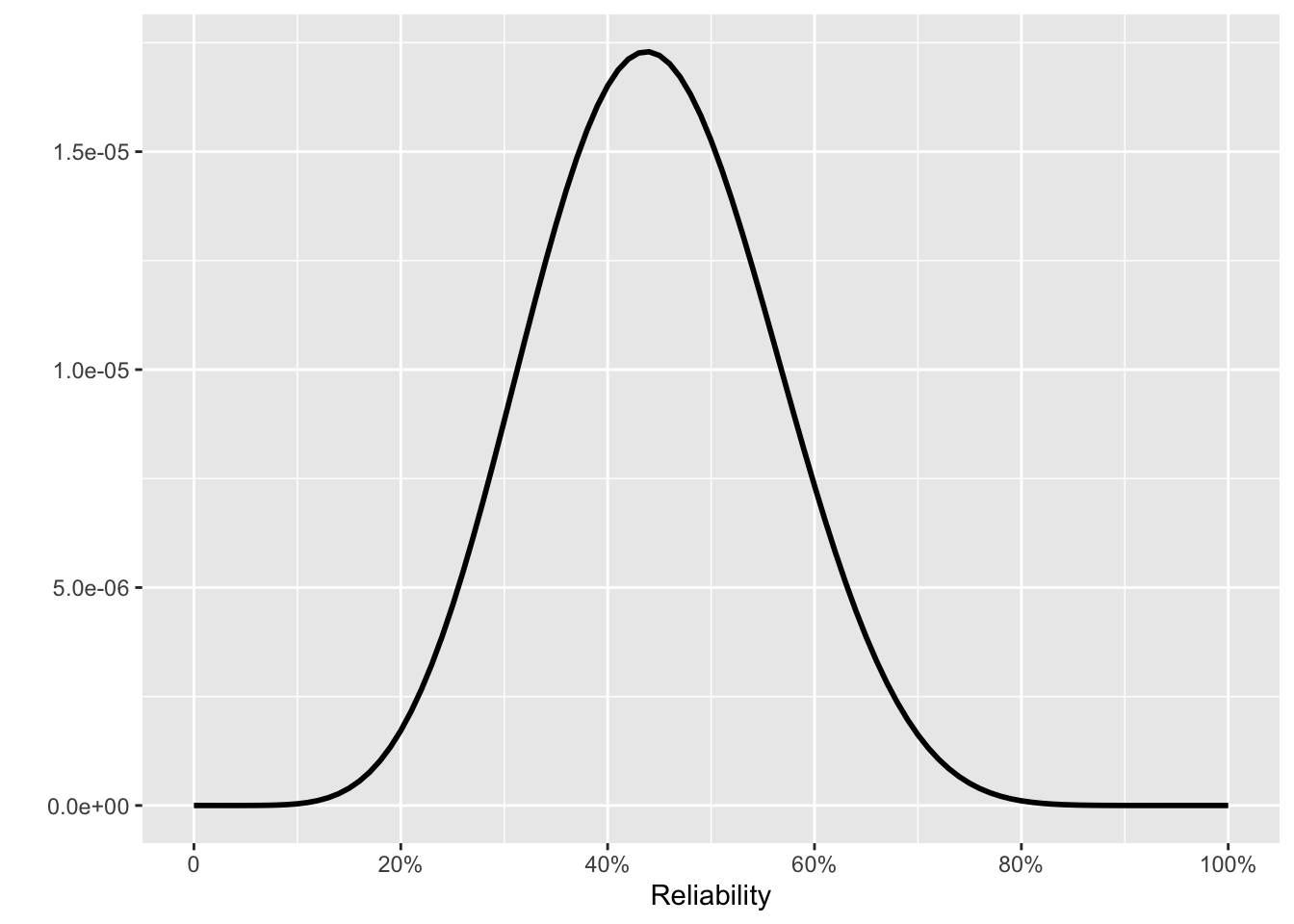
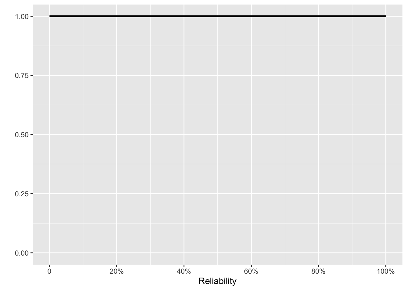
To find that sensible prior, go back to the time before the first 16 tests. Lacking tests, we have no information. However, “no information” reasonably corresponds to a prior that assigns equal weight to every reliability value between 0% and 100%. In other words, the original prior, before the 16 tests, is a uniform distribution.
The prior for the last four tests of the 20 tests is the posterior after the first 16. Calculating that posterior means multiplying, for each of the 16 tests, by the likelihood corresponding to a success or failure. The success and failure likelihoods have simple forms.
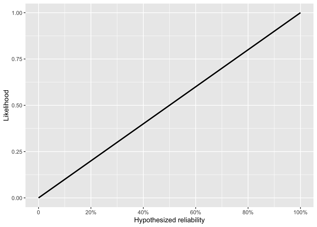
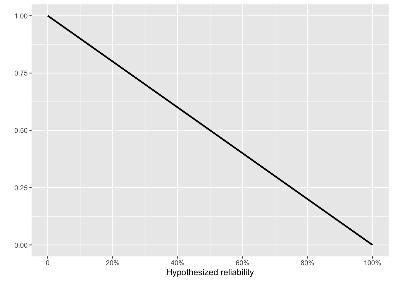
With the likelihood functions for each of the first 16 tests applied, we can calculate a reasonable prior to use when analyzing the last four tests.
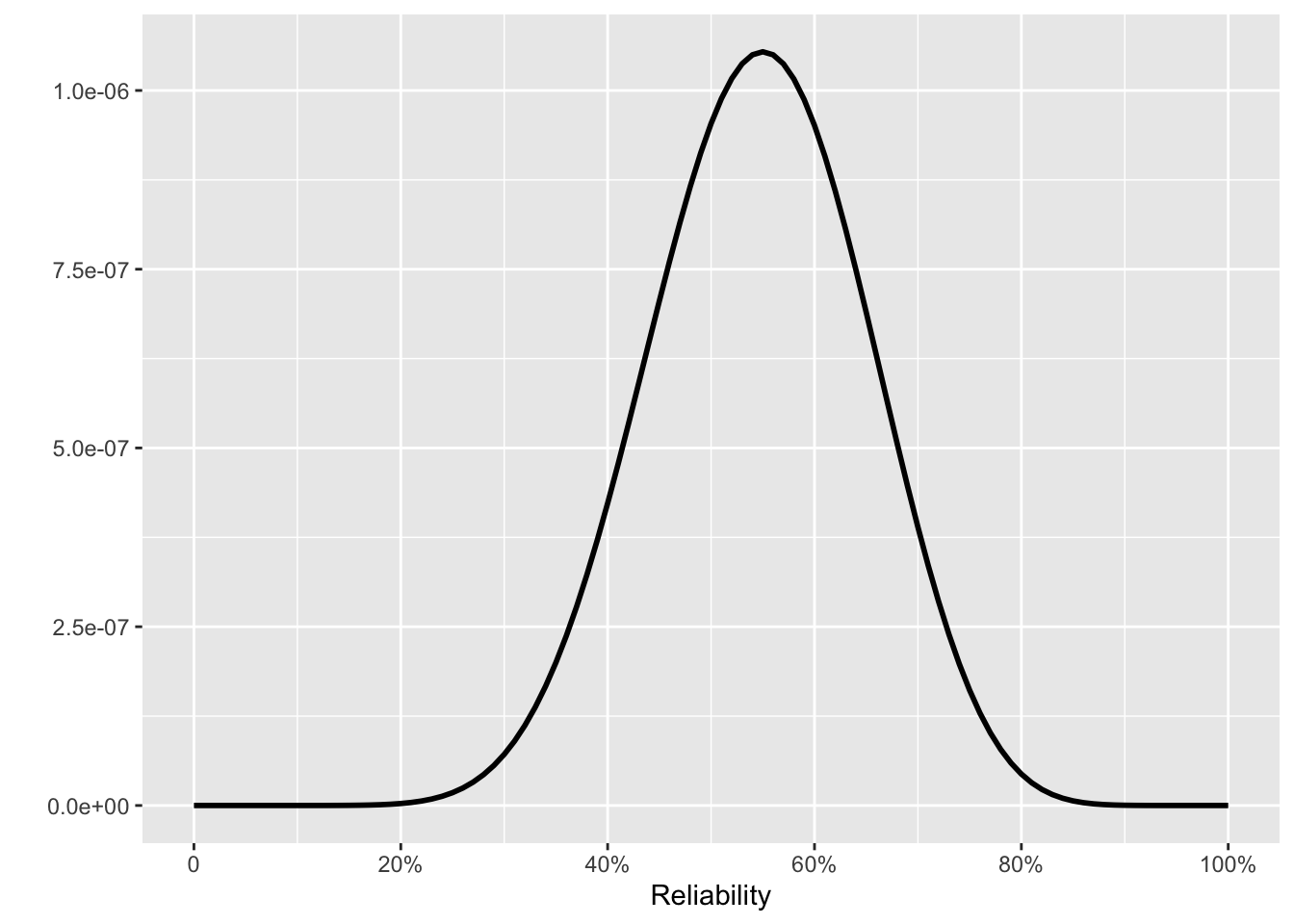
We start with a prior for our beliefs before performing any tests. It may sound odd to calculate a prior by assuming a prior. But remember that the purpose of ☞ Bayesian multiplication ☜ is to update a prior to a posterior. That posterior then becomes a new prior for analyzing new data. Fig 10. 5 shows snapshots of the posteriors at several points in the 16 tests.
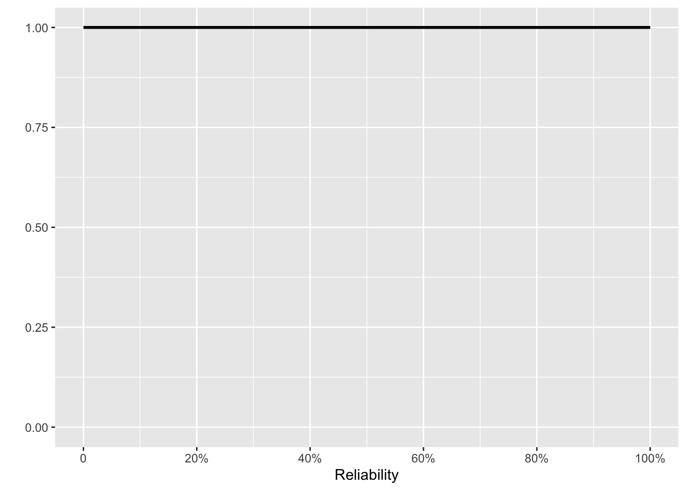
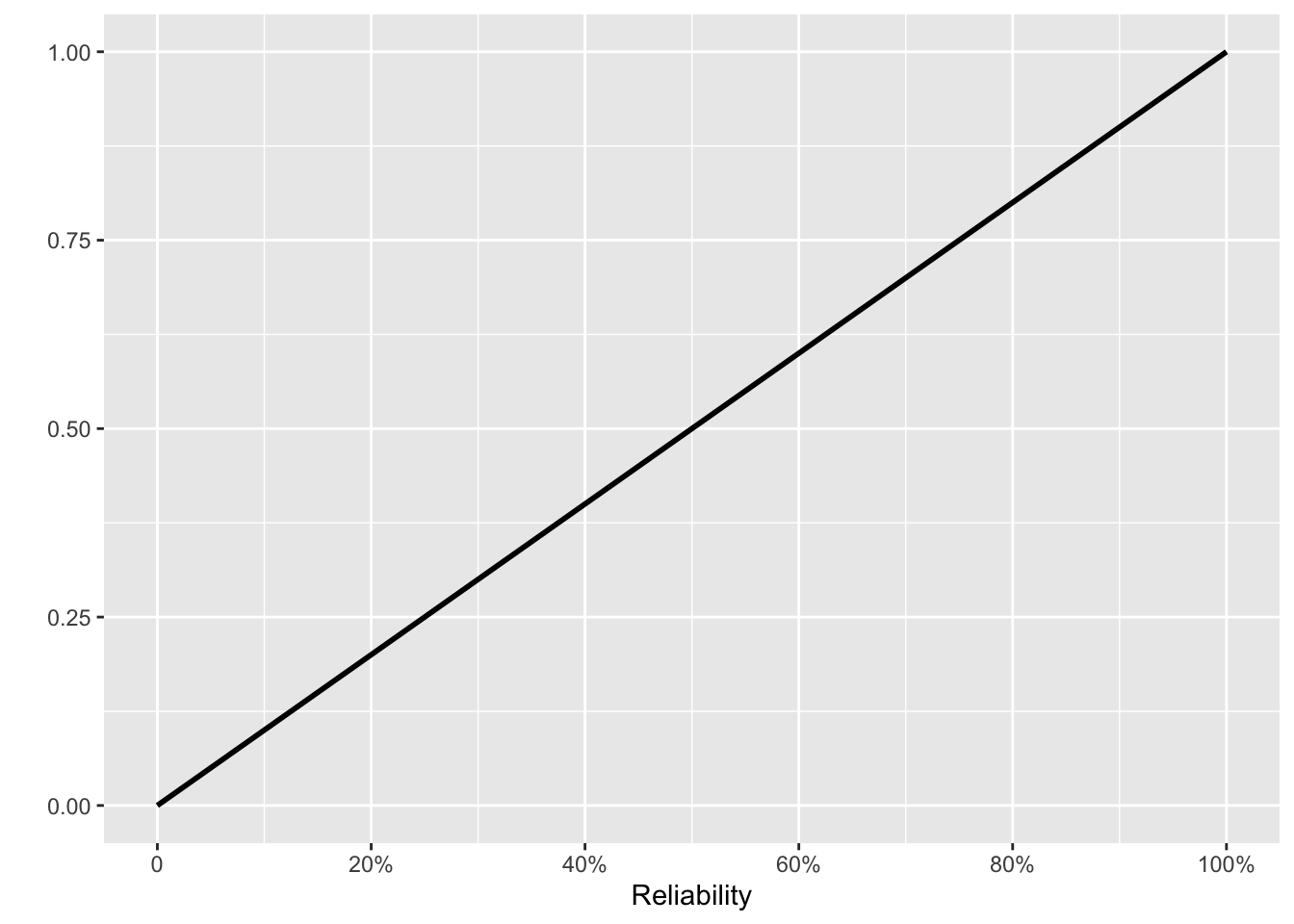
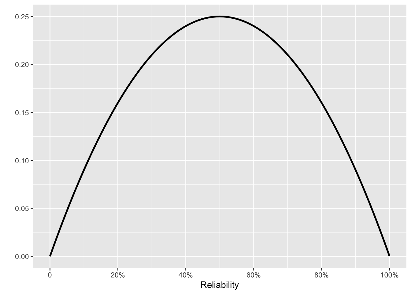
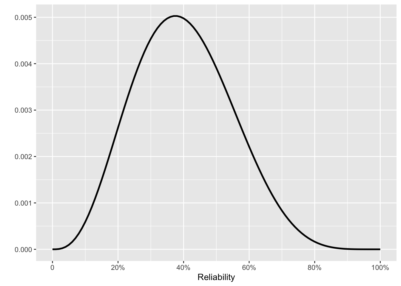
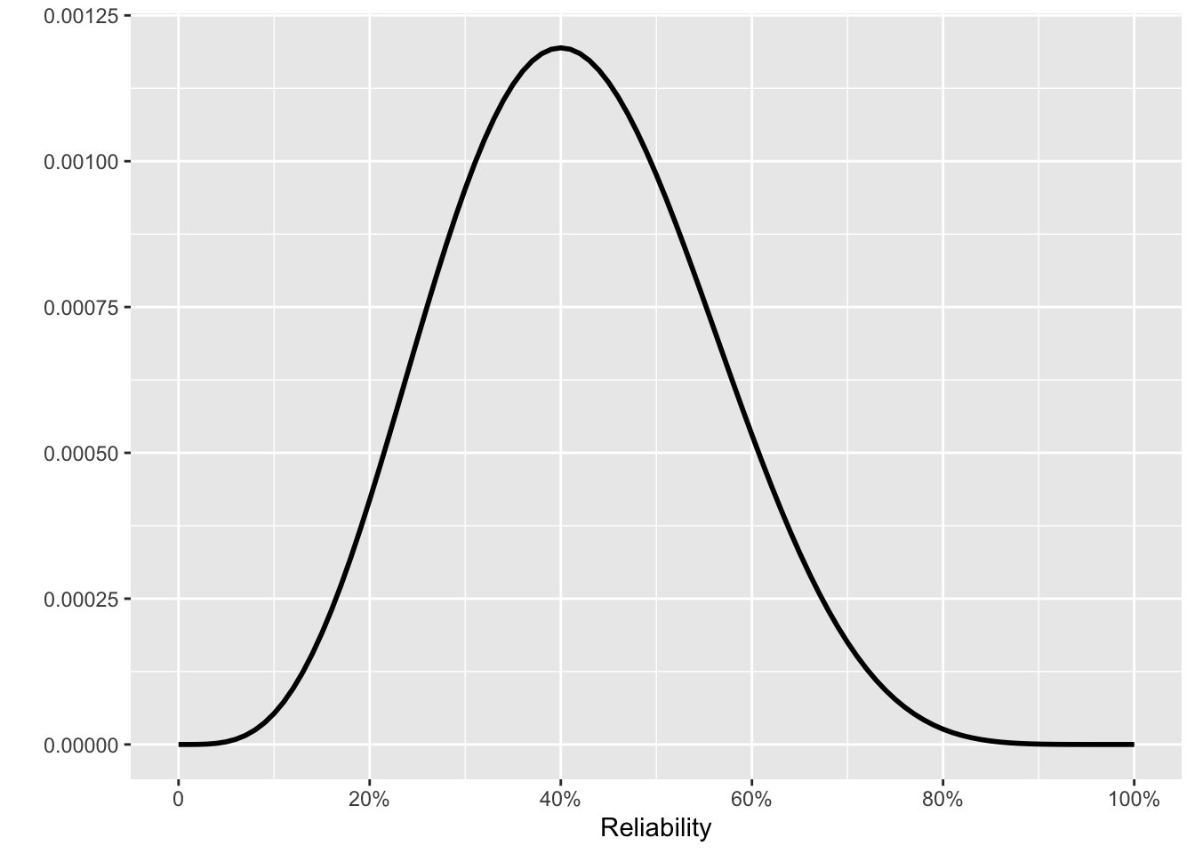
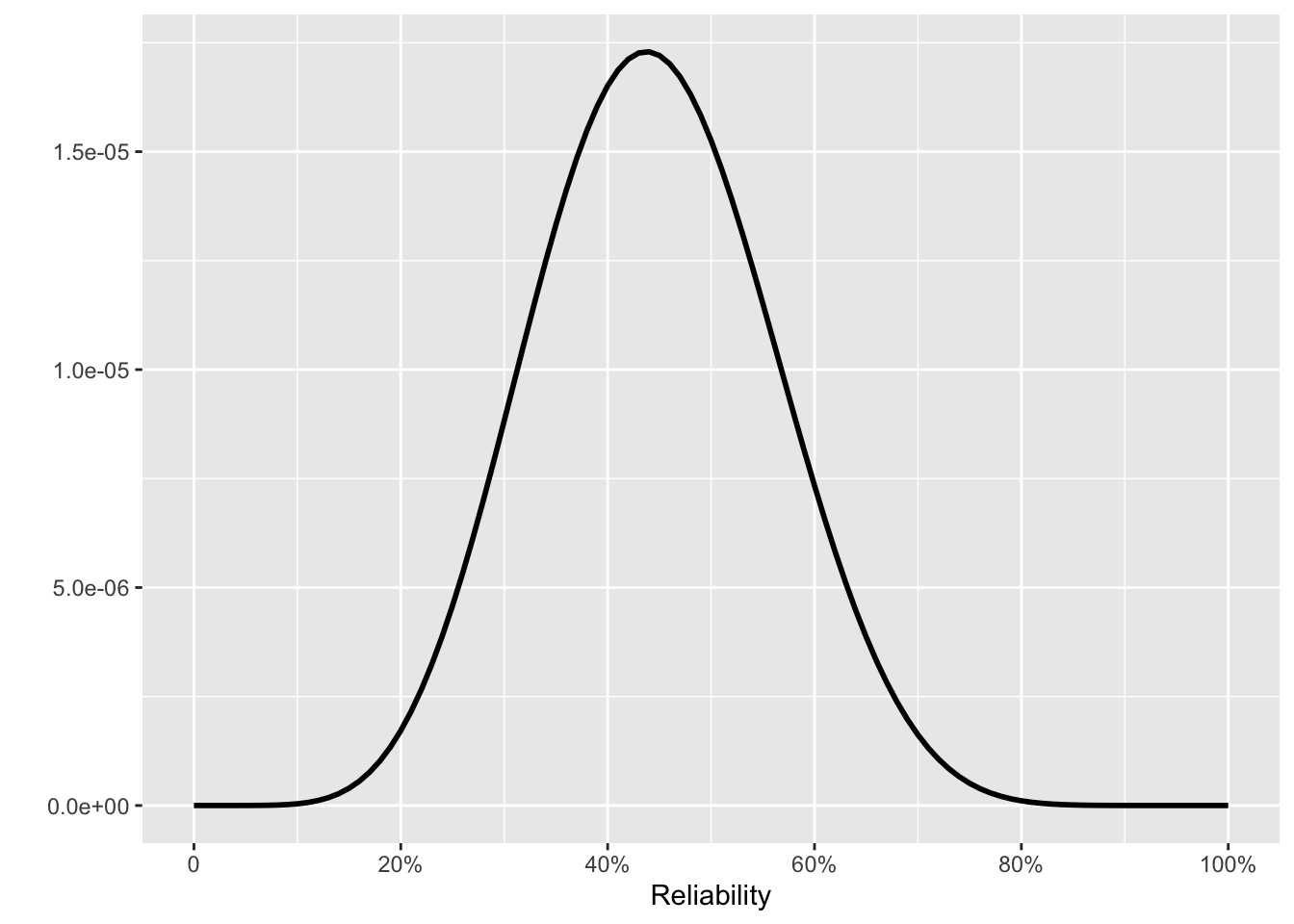
We set the initial prior to be flat: all levels of reliability are equally probable. Thereafter, each new test is the posterior from the previous test multiplied by one of Fig 10. 4 (a) or (b), depending on whether that test was a success or failure.
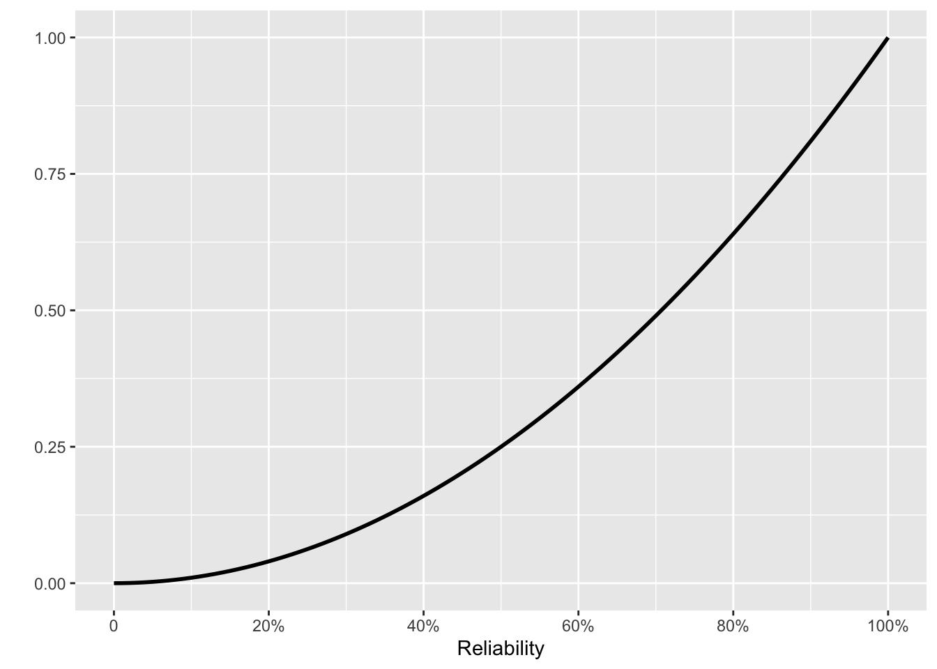
On to the next four tests, which were all successful. What kind of reliability claim does this support? Fig 10. 6 shows some reasonable possibilities.
Using the posterior from the first 16 tests as the prior, the next 4 successful tests lead us to the posterior in Fig 10. 6(d).
It wouldn’t be outrageous to argue for a different prior. Perhaps the Pentagon insists, “This new technology is completely different and much better from the old stuff used in the earlier 16 tests. Let’s start fresh with a flat prior.” This produces the posterior in Fig 10. 6(e).
Or perhaps the Pentagon is more aggressive. “The new stuff is really good. Simulations show it working all the time. We propose the prior in Fig 10. 6(e).” The resulting posterior is shown in Fig 10. 6(f).
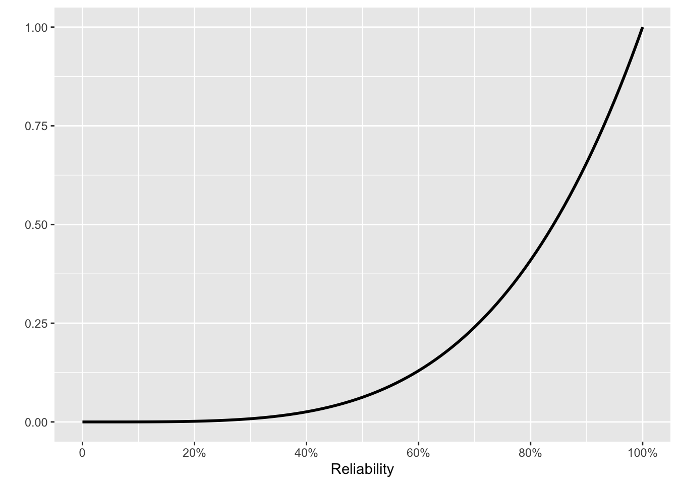
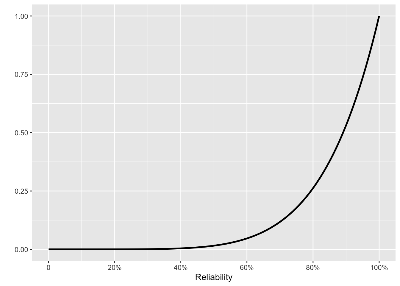
It can be unsettling at first to express the success rate as a distribution rather than a single number. A single number would sound more authoritative. But such authority is unjustified: the data cannot support an isolated claim of a success rate. The novelist F. Scott Fitzgerald wrote a line that reflects the genuine uncertainty: “The test of a first-rate intelligence is the ability to hold … opposed ideas in the mind at the same time, and still retain the ability to function.” Even the most favorable prior (Fig 10. 6(c)) gives some credibility to the belief that the reliability is around 60%. The posterior from that prior (Fig 10. 6(f)) continues to assign a probability of one-fourth to the possibility that the reliability is 80% or lower.
The Pentagon’s claim of 100% reliability does indeed find some support from the posterior distribution. However, “some support” does not constitute effective planning for dealing with the possibility of an attack.3