Instructor Teaching Notes for Lesson 29

Math300Z

Author

Daniel Kaplan

Published

March 8, 2023

See Takeaways from Lesson 28 for a review of the last class. There, we introduced the term “covariate” to describe an explanatory variable that isn’t of direct interest but which might be important to how the system being modeled works.

hospital_dag <- dag_make(
  size ~ binom(1+exo(), labels=c("small", "large")),
  severity ~ 1+ exo() - 2*I(size=="small"),
  outcome ~ binom(-1 + severity + I(size=="small"), labels=c("good", "bad"))
)
patients <- sample(hospital_dag, size=1000)

stats <- patients |> group_by(size) |>
  summarize(msevere=mean(severity), bad = mean(outcome=="bad"))
stats

# A tibble: 2 × 3
  size  msevere   bad
  <chr>   <dbl> <dbl>
1 large   0.997 0.469
2 small  -0.939 0.311

mod1 <- model_train(zero_one(outcome, one="bad") ~ size, 
                    data=patients)
model_plot(mod1, x=severity, color=size, data_alpha=0.02) |>
  gf_point(bad ~ msevere, color=~size, data=stats)

Warning: Ignoring unknown aesthetics: fill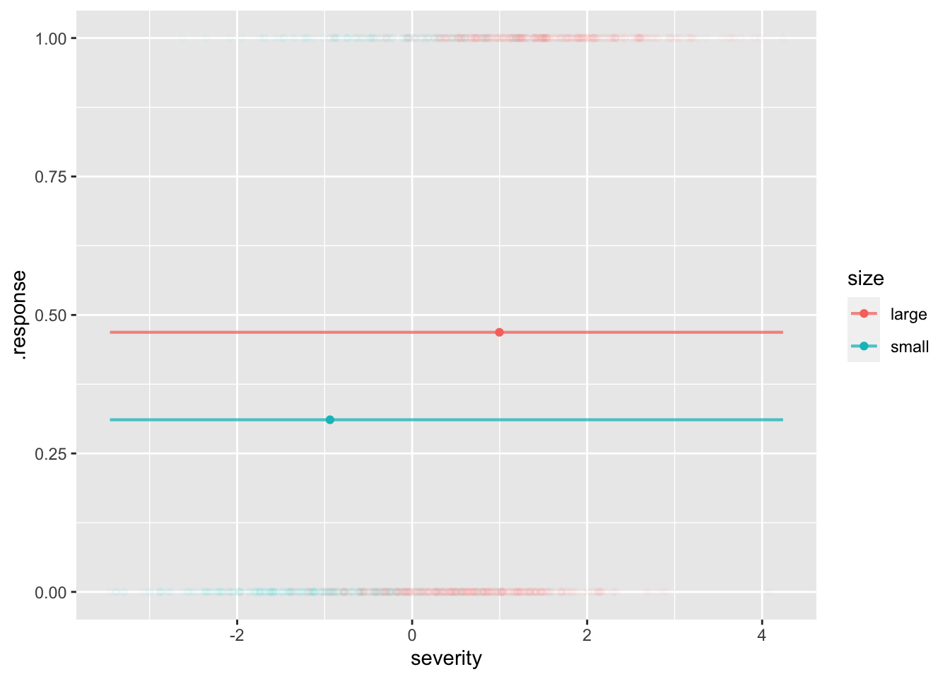

mod2 <- model_train(zero_one(outcome, one="bad") ~ size*severity, 
                    data=patients)
model_plot(mod2, x=severity, color=size, data_alpha=0.02) |>
  gf_point(bad ~ msevere, color=~size, data=stats)

Warning: Ignoring unknown aesthetics: fill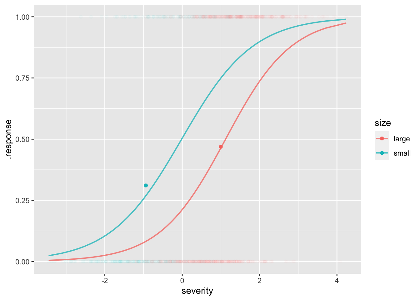

Adjusting for severity …

model_eval(mod2, severity=0, size=c("small", "large"),
           interval="confidence")

  severity  size   .output      .lwr      .upr
1        0 small 0.5039882 0.4205391 0.5872158
2        0 large 0.2122228 0.1701288 0.2614506

The effect size w.r.t. an explanatory variable is automatically adjusted for all the covariates.

Class activity

Adjusting for age

“Life tables” are compiled by governments from death certificates.

LTraw <- readr::read_csv("life-table-raw.csv")

Rows: 120 Columns: 7
── Column specification ────────────────────────────────────────────────────────
Delimiter: ","
dbl (7): age, male, mnum, mlife_exp, female, fnum, flife_exp

ℹ Use `spec()` to retrieve the full column specification for this data.
ℹ Specify the column types or set `show_col_types = FALSE` to quiet this message.

head(LTraw)

# A tibble: 6 × 7
    age     male   mnum mlife_exp   female   fnum flife_exp
  <dbl>    <dbl>  <dbl>     <dbl>    <dbl>  <dbl>     <dbl>
1     0 0.00584  100000      74.1 0.00491  100000      79.8
2     1 0.00041   99416      73.6 0.000316  99509      79.2
3     2 0.000254  99376      72.6 0.000196  99478      78.2
4     3 0.000207  99350      71.6 0.00016   99458      77.2
5     4 0.000167  99330      70.6 0.000129  99442      76.2
6     5 0.000141  99313      69.6 0.000109  99430      75.2

Wrangling to a more convenient format (for our purposes):

LT <- tidyr::pivot_longer(LTraw |> select(age, male, female), c("male", "female"), names_to="sex", values_to="mortality")
LT

# A tibble: 240 × 3
     age sex    mortality
   <dbl> <chr>      <dbl>
 1     0 male    0.00584 
 2     0 female  0.00491 
 3     1 male    0.00041 
 4     1 female  0.000316
 5     2 male    0.000254
 6     2 female  0.000196
 7     3 male    0.000207
 8     3 female  0.00016 
 9     4 male    0.000167
10     4 female  0.000129
# … with 230 more rows

Age pyramids comparing the US population in 1972 and 2021

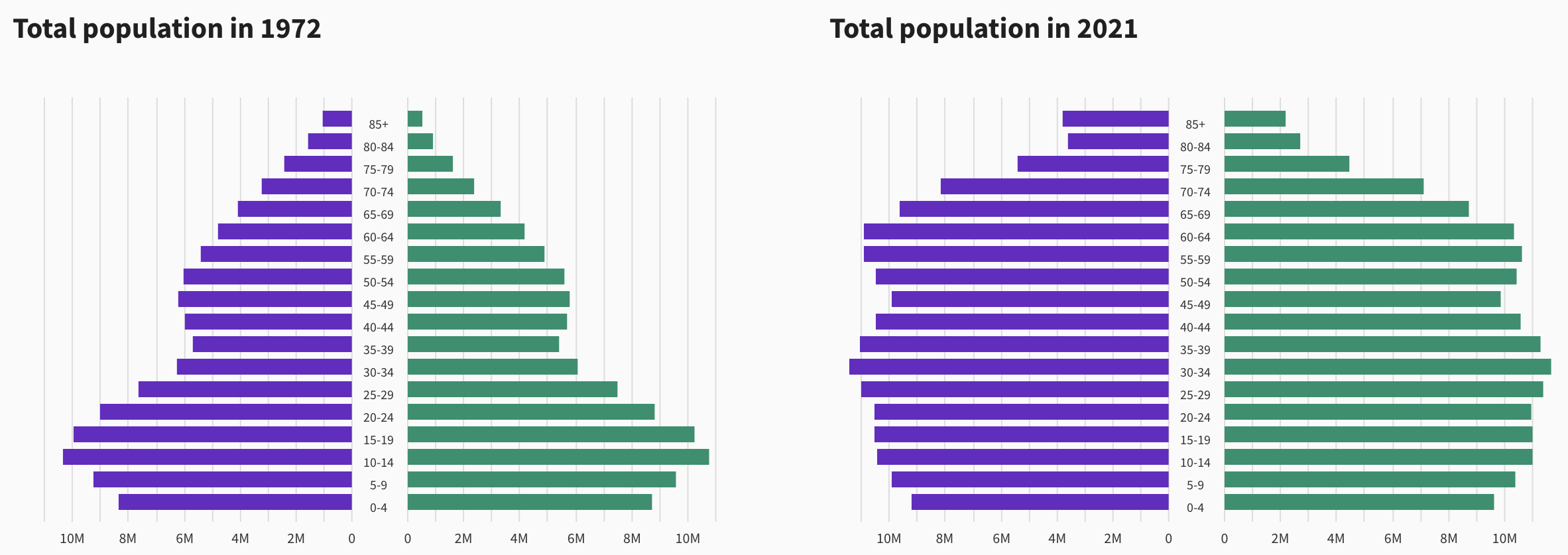
Questions:

When were people aged 35-39 in 1972 born? Why are there so few of them?
How old would you have to be in 1972 to be part of the “baby boom?” Can you see the echo of the baby boom in 2021?
How many 85+ year-olds will there be in 2040?

The raw data:

Code

Pop2020 <- readr::read_csv("nc-est2021-agesex-res.csv",
                           show_col_types=FALSE) |>
  filter(SEX > 0, AGE<999) |>
  mutate(sex = ifelse(SEX==1, "female", "male"), 
         age=AGE, pop=ESTIMATESBASE2020) |> 
  select(age, sex, pop)

Pop2020 |> tail()

# A tibble: 6 × 3
    age sex      pop
  <dbl> <chr>  <dbl>
1    95 male  132299
2    96 male  105435
3    97 male   79773
4    98 male   57655
5    99 male   43072
6   100 male   78474

US mortality at actual age distribution involves joining the data from these two data frames.

Overall <- Pop2020 |> left_join(LT)

Joining, by = c("age", "sex")

head(Overall)

# A tibble: 6 × 4
    age sex        pop mortality
  <dbl> <chr>    <dbl>     <dbl>
1     0 female 1907982  0.00491 
2     1 female 1928926  0.000316
3     2 female 1980392  0.000196
4     3 female 2028781  0.00016 
5     4 female 2068682  0.000129
6     5 female 2081588  0.000109

The calculation is simple wrangling:

Overall |> group_by(sex) |>
  summarize(mortality = 100000*sum(pop*mortality)/sum(pop))

# A tibble: 2 × 2
  sex    mortality
  <chr>      <dbl>
1 female      708.
2 male       1351.

The WHO standard age distribution

Code

Raw <- readr::read_csv("who-standard-age-distribution.csv",
                            show_col_types=FALSE)
Tmp <- Raw |> mutate(mid = (high+low)/2)
popfun <- approxfun(Tmp$mid, Tmp$pop, yleft=8.860, yright=0.04)
Standard <- tibble(
  age = 0:99,
  pop = popfun(age)
)
ggplot(Standard, aes(xmin=-pop, xmax=pop, y=age)) + geom_ribbon(alpha=.3, aes(xmin=0), fill="green") + 
  geom_ribbon(alpha=.3, aes(xmax=0), fill="blue")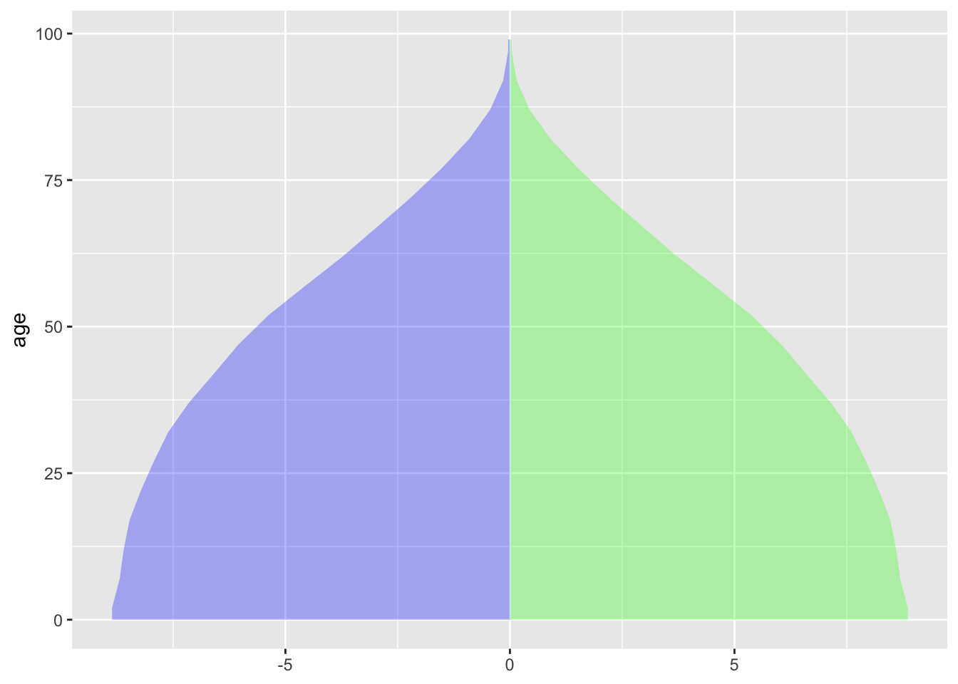

US mortality at WHO standard age distribution:

Overall <- Standard |> left_join(LT)

Joining, by = "age"

Overall |> group_by(sex) |>
  summarize(mortality = 100000*sum(pop*mortality)/sum(pop))

# A tibble: 2 × 2
  sex    mortality
  <chr>      <dbl>
1 female      439.
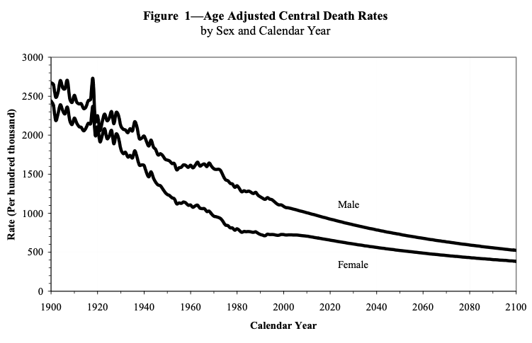
2 male        681.

Age-adjusted death rates over time

From the SSA (p. 15)