Galton |> names()[1] "family" "father" "mother"
[4] "sex" "height" "nkids" Recall the three kinds of computational objects that we work with:
In this activity we will relate these one to the other, in the process building up an intuitive understanding of regression.
Note that this is intended for instructors; it is highly streamlined from the version that students see.
As a running example, we’ll work with the data Francis Galton collected in the 1880s about the heights of children and their parents. This dataset was instrumental in the invention of the correlation coefficient and the notion of “regression to mediocrity.”
The data frame, Galton, is provided by the {mosaicData} package.
Galton, like data frames from other package, is available via the command ?Galton.
height and sex of the child, the heights of the child’s mother and father, and the number of children in the family (nkids).In R, everything you do involves a function call. Invoking a function is accomplished by following the function name by a pair of parentheses.
We use the pipeline style of constructing most commands. This uses the |> token, which can never be at the start of a line. Most often, the “wellhead” for the pipeline is a data frame, but it can also be a regression model or a graphic.
The names of simple functions to look at the contents of a data frame include head(), nrow(), and names(). If you are working in the RStudio interface (not the web app!), you can also use View().
Galton |> names()[1] "family" "father" "mother"
[4] "sex" "height" "nkids" Galton |> nrow()[1] 898Galton |> head() family father mother sex height nkids
1 1 78.5 67.0 M 73.2 4
2 1 78.5 67.0 F 69.2 4
3 1 78.5 67.0 F 69.0 4
4 1 78.5 67.0 F 69.0 4
5 2 75.5 66.5 M 73.5 4
6 2 75.5 66.5 M 72.5 4The re-organization and transformation of data is called “data wrangling.” We use a small set of wrangling function extensively in the Lessons.
Several other wrangling functions are demonstrated but not needed to follow the Lessons. These include
mutate() creates new variables from existing onesgroup_by() sets up data frames so that successive wrangling operations work in a groupwise manner.summarize() reduces a multi-row data frame into a single row data frame (more generally, a single row for each group).arrange()select() dismisses variables that are not needed for successive wrangling operations.filter() dismisses rows that don’t meet a specified criterion.Wrangling functions always take a data frame as the first argument/input and produce a data frame as the output. Other arguments are used to specify details of the wrangling operation.
In this workshop, we’ll use mutate(), summarize(), and group_by(). It us easier to read the wrangling expressions if you can keep three things in mind:
Galton |>
  summarize(mn = mean(height),
            s = sd(height),
            count=n())
mn s count
1 66.76069 3.582918 898Galton |>
group_by(sex) |>
summarize(mn = mean(height),
s = sd(height),
count=n())# A tibble: 2 × 4
sex mn s count
<fct> <dbl> <dbl> <int>
1 F 64.1 2.37 433
2 M 69.2 2.63 465Note that the argument(s) to group_by() are practically always one or more categorical variables. Let’s see what happens when a numerical variable is used with group_by().
Try the second of the above commands, but replace categorical sex with quantitative mother. Explain what’s happening. Also explain why sometimes the standard deviation is missing (NA).
var(), sd(), mean(), n() and so on.name = value or operation
For instance, here are wrangling expressions to do the kind of calculations often encountered in Stat 101. We won’t need such calculations very often in Lessons but they are nice to start with a context that students will already be familiar with:
mutate: add or modify a variable
The mutate() wrangling operation is done on a row-by-row basis. Example: Galton, lacking a method to work with multiple explanatory variables had to combine the mother and father heights into a single quantity: midparent.
midparent since it’s the average of the mother’s and father’s heights.
family father mother sex height nkids midparent
1 1 78.5 67.0 M 73.2 4 72.75
2 1 78.5 67.0 F 69.2 4 72.75
3 1 78.5 67.0 F 69.0 4 72.75
4 1 78.5 67.0 F 69.0 4 72.75
5 2 75.5 66.5 M 73.5 4 71.00
6 2 75.5 66.5 M 72.5 4 71.00:::
:::
Most Stat 101 instructors would see summarize() as the route to topics like the one- and two-sample t-tests. After all, this command gives the raw ingredients that go into the t-test calculation.
Galton |>
  group_by(sex) |>
  summarize(mn = mean(height),
            s = sd(height),
            count=n())
# A tibble: 2 × 4
sex mn s count
<fct> <dbl> <dbl> <int>
1 F 64.1 2.37 433
2 M 69.2 2.63 465All that’s needed is to pull out the values from this data frame and plug them into the t-test formula. Doing this task in R involves tedious and frustration-inducing programming, the sort that leads students to pull out their graphing calculators and instructors to question whether computers are genuinely helpful in teaching intro stats.
The short-cut involves using a black box, e.g. this widely used R command:
t.test(height ~ sex, data=Galton, var.equal=TRUE)
    Two Sample t-test

data:  height by sex
t = -30.548, df = 896, p-value < 2.2e-16
alternative hypothesis: true difference in means between group F and group M is not equal to 0
95 percent confidence interval:
 -5.447513 -4.789798
sample estimates:
mean in group F mean in group M
       64.11016        69.22882
We will NOT follow this path. One simple reason is that the output of t.test() is not a data frame nor any other sort of general-purpose computer object.
We only want to work with three kinds of objects: data frame, regression model, graphics.
A more fundamental reason to eschew t.test() and its ilk is the need to generalize. For instance, we want to be able to study covariates and causality, but t.test() provides no direct route for including covariates.
The first step on the modeling path is “model values.” Models can be seen as simplifications of the data (useful for the purpose of summary).
mutate() rather than summarize().Mod_galton <- Galton |>
group_by(sex) |>
mutate(modval = mean(height)) |>
ungroup()head(Mod_galton)# A tibble: 6 × 7
family father mother sex height nkids modval
<fct> <dbl> <dbl> <fct> <dbl> <int> <dbl>
1 1 78.5 67 M 73.2 4 69.2
2 1 78.5 67 F 69.2 4 64.1
3 1 78.5 67 F 69 4 64.1
4 1 78.5 67 F 69 4 64.1
5 2 75.5 66.5 M 73.5 4 69.2
6 2 75.5 66.5 M 72.5 4 69.2Why are there just two values in the modval column?
Graphics can be used to show the “shrinkage.”
Since students would not be expected to make such a graph, I’ve hidden the code. You can open it up if you like.
Mod_galton |> sample(size=50) |>
  gf_point(height ~ sex,
          alpha=0.3,
          position = position_jitter(height=0, seed=101)) |>
          gf_point(modval ~ sex, height=0, color="blue",
position = position_jitter(height=0, seed=101)) 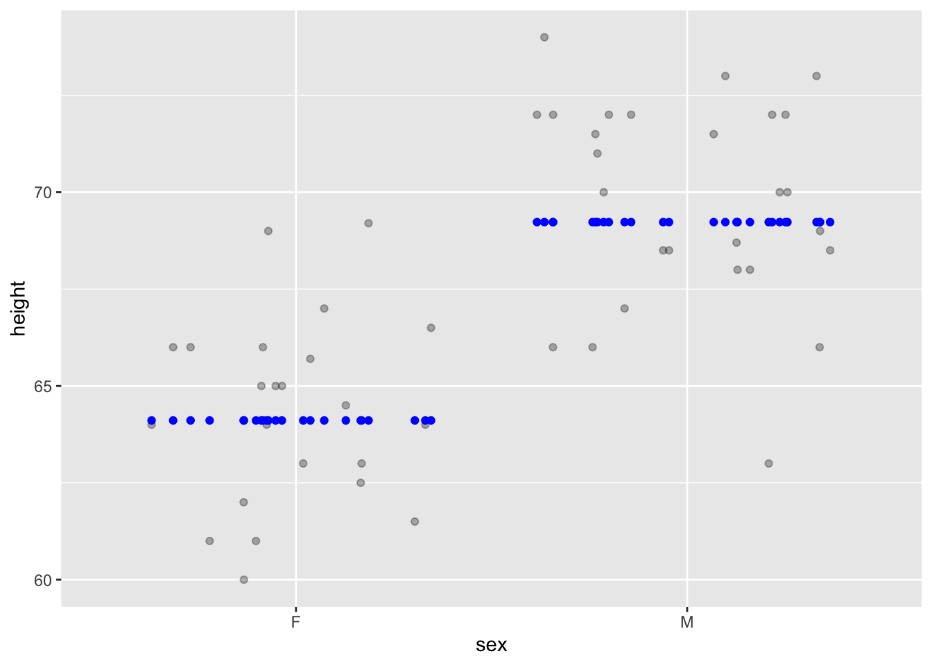
We measure the amount of variation with the variance.
Try the above with sd() instead of var(). Does the standard deviation split the total into two parts that add up to the whole?
Mod_galton |>
  summarize(vtotal=var(height),
            vfitted=var(modval),
            vresid=var(height - modval),
            R2=vfitted/vtotal)
# A tibble: 1 × 4
vtotal vfitted vresid R2
<dbl> <dbl> <dbl> <dbl>
1 12.8 6.55 6.29 0.510The variance of the response variable is split into two parts: that ascribed to the explanatory variable(s) and the leftover (“residual”) variance.
I didn’t do this in Lessons, but perhaps I should have. Tell me what you think.
In some situations it’s doubtful whether an explanatory variable is providing any geniune “explanation” of the variation in the response. Perhaps it’s just a matter of chance. We can test this hypothesis by replacing the explanatory variable by one that is just a matter of chance.
Galton |>
  mutate(random = shuffle(sex)) |>
  group_by(random) |>
  mutate(modval = mean(height)) |>
  ungroup() |>
  summarize(vtotal = var(height),
            vfitted = var(modval),
            vresid = var(height - modval),
            R2 = vfitted/vtotal)
?(caption)
# A tibble: 1 × 4
  vtotal vfitted vresid       R2
   <dbl>   <dbl>  <dbl>    <dbl>
1   12.8 0.00413   12.8 0.000322
[Motivation] Help the students intuit the idea of a continuous function.
Before showing the class what happens when we group_by(mother), ask them to speculate what the relationship between mother’s and child’s height might be.
Translate their answers into a graphical sketch: “child’s tendency” versus mother’s height.
What happens if we use a numerical explanatory variable with group_by()? Let’s try! We’ll use mother as the explanatory variable.
Mod2galton <-
  Galton |>
  group_by(mother) |>
  mutate(modval = mean(height)) |>
  ungroup()
Looking at the results graphically:
Mod2galton |>
  gf_point(height ~ mother, alpha=0.1) |>
  gf_point(modval ~ mother, color="blue", size=2) |>
  gf_line(modval ~ mother, color="blue")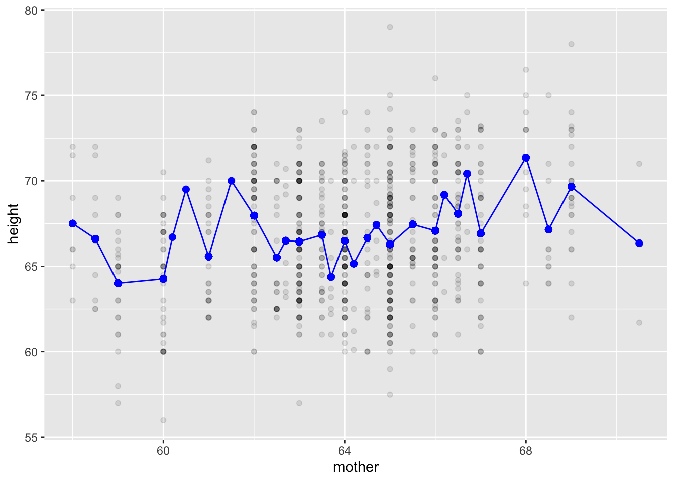
What strikes you as implausible about this model of the relationship between mother’s height and child’s height?
The height of the mother isn’t the only variable that it’s plausible to think is connected to (full-grown) child’s height. How about father and sex of the child. Let’s add in sex as another explanatory variable.
Mod3galton <-
  Galton |>
  group_by(mother, sex) |>
  mutate(modval = mean(height)) |>
  ungroup()
Mod3galton |>
  gf_point(height ~ mother, alpha=0.1, color=~sex) |>
  gf_point(modval ~ mother, color=~sex, size=2) |>
  gf_line(modval ~ mother, color=~sex)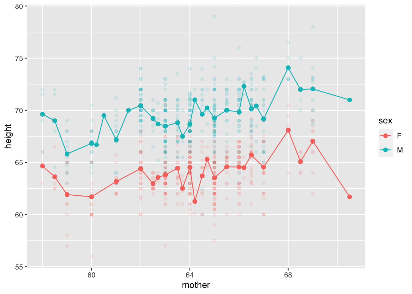
mother and the child’s sex as explanatory variables.
We’d like a simpler pattern to the relationship. How might we accomplish this?
mother into groups: short and tall.Mod_ii_galton <-
Galton |>
group_by(ntile(mother,3), sex) |>
mutate(modval = mean(height)) |>
ungroup()
Mod_ii_galton |>
gf_point(height ~ mother, alpha=0.1) |>
gf_point(modval ~ mother, color=~sex, size=2) |>
gf_line(modval ~ mother, color=~sex)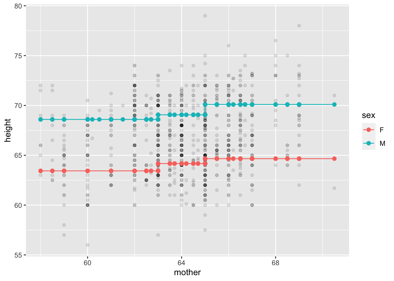
mother into three groups for the purpose of modeling.For both females and males and males, the difference in average child’s height between the shorter third of mothers and the taller third is about 1.25 inch.
The breaks between adjacent line segments are an artifact of the method. It would be nice to remove this artifact. To do so, we want to avoid splitting up the mothers into distinct groups, i. but allow the effect of mother to show continuous change. ii. Replace mean() with the model_values() function, whose output can vary continuously with mother.
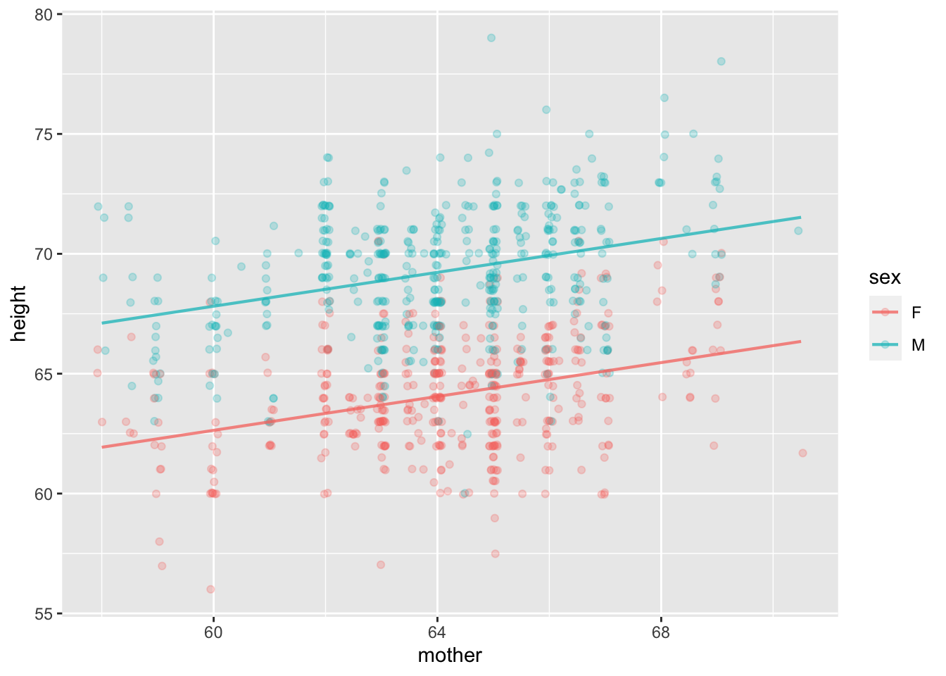
1Mod_iii_galton <- Galton |>
  group_by(sex) |>
2  mutate(modval = model_values(height ~ mother)) |>
ungroup()height) and the explanatory variable (mother).
Mod_iii_galton |>
  gf_point(height ~ mother, alpha=0.1) |>
  gf_point(modval ~ mother, color=~sex, size=2) |>
  gf_line(modval ~ mother, color=~sex)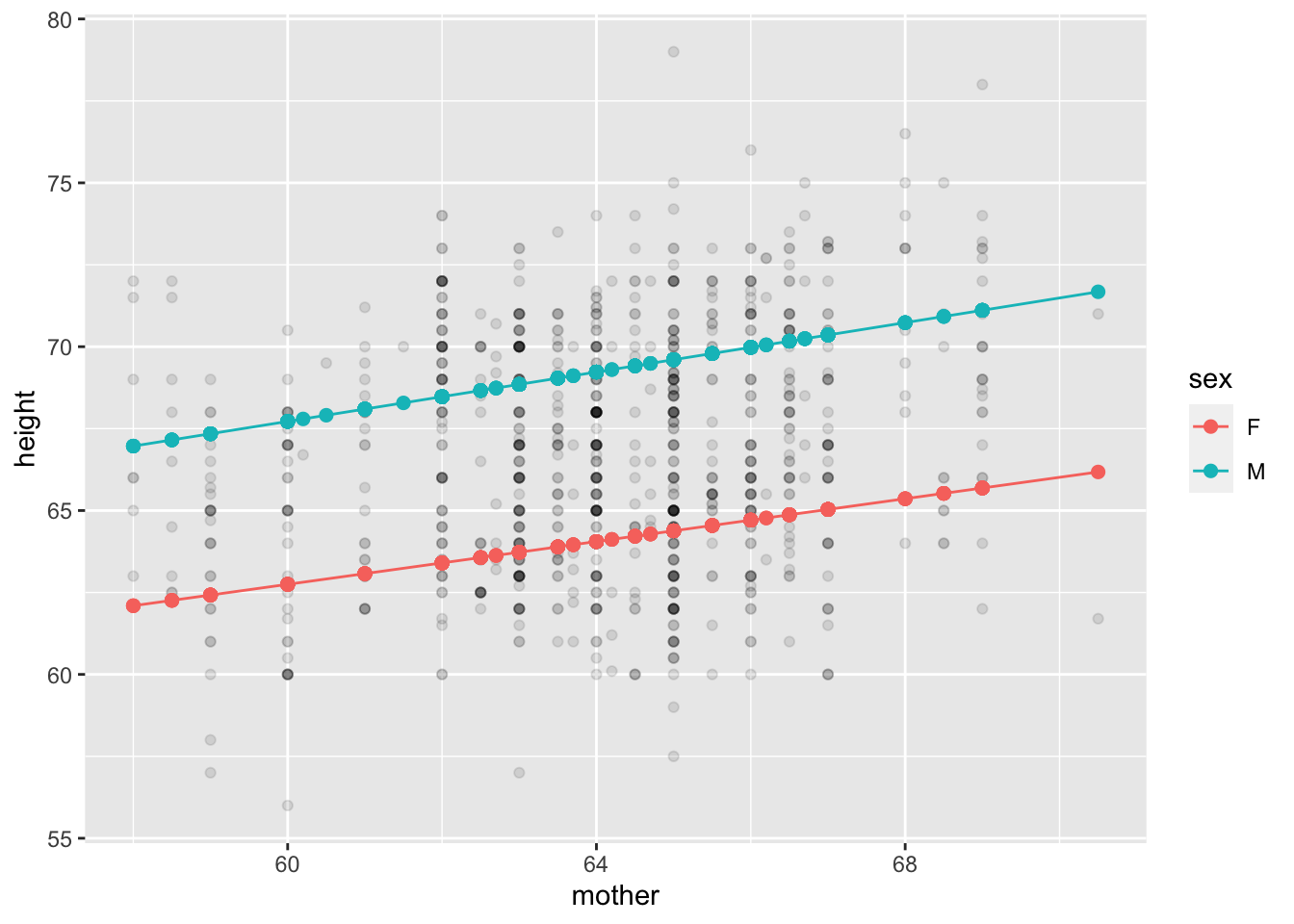
mother.The argument to model_values() is height ~ mother. This says that we want to model height as a function of mother.
model_values() can allow multiple explanatory variables. Modify the previous chunk to eliminate the group_by() stage entirely and set the model values using model_values(height ~ mother + sex).
This third step in our exploring modeling ended up with a lot of code. In the fitting and graphing commands, the variable mother appears in 4 places; height appears in another 4; sex in 3 places and modval in 3.
The only essential information that goes into the Step-3 code is:
Galton.height ~ mother + sexWe want to simplify the process considerably. We’ll do that by using another (equivalent) model-training function that keeps track of the response and explanatory variables for the graphing and summarization stage.
We will use model_train() for the rest of the course. You won’t need the mutate(), summarize(), or model_values() functions.
Mod <- Galton |> model_train(height ~ mother + sex)
Mod |> model_plot()
Mod |> R2() n k Rsquared F adjR2 p df.num df.denom
1 898 2 0.5618019 573.7276 0.5608227 0 2 895For technical reasons, model_train() does not produce a data frame. Instead, the object produced by model_train() is a different kind of object: a model.
lm, but this is not important to our purposes.Let’s extend the model of height to include the father. And make another model with perhaps another factor, the size of the family.
Mod2 <- Galton |> model_train(height ~ mother + sex + father)
Mod3 <- Galton |> model_train(height ~ mother + sex + father + nkids)
The graph of the models are more complicated because they have three (or four) explanatory variables. For instance:
It’s hard to interpret the plot of Mod2, especially any trend with father. As is often the case, re-arranging which variable is used for which aesthetic can give a different view. The three aesthetics here are x=, color=, and facet=. Try different combinations of mother, father, and sex to create a plot of the model that’s easier to interpret.
model_plot(Mod2, x = _____, color = _____, facet = _____)model_plot(Mod2)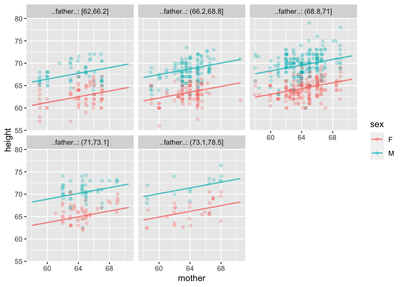
Mod3 includes a fourth explanatory variable, nkids. Including this might be because we hypothesize that, say, in bigger families there is less food per child, or that in bigger families there is more chance to catch a contagious disease. Both these factors can stunt growth in children.
Mod |> R2() n k Rsquared F adjR2 p df.num df.denom
1 898 2 0.5618019 573.7276 0.5608227 0 2 895Mod2 |> R2() n k Rsquared F adjR2 p df.num df.denom
1 898 3 0.6396752 529.0317 0.6384661 0 3 894Mod3 |> R2() n k Rsquared F adjR2 p df.num df.denom
1 898 4 0.640721 398.1333 0.6391117 0 4 893One way to test whether nkids is contributing to the model is to compare the R2 both with and without the nkids term.
Adding father to the height ~ mother + sex model increases the R2 by about 7 percentage points.
Adding nkids to height ~ mother + sex + father increases R^2 by only 0.4 percentage points. If nkids is contributing to height, it’s only by a small amount.