Statistical entities
Running with George Cobb’s metaphor of the tear-down … Let’s imagine what the new building will look like.
Start with the kitchen, the place where raw ingredients (data, beliefs) get turned into nutritious information.
At its most basic, a kitchen contains a small set of standard appliances, each of which a cook knows how to operate: refrigerator, stove, oven, sink, pans, knives, cutting board, trash can. For an introduction to kitchen operations, I propose to start with a very small set, small enough that the student can keep them all in mind. Or, more philosophically,
Entia non sunt multiplicanda praeter necessitatem.—William of Occam (1285-1346)
Alles muß so einfach wie möglich sein. Aber nicht einfacher.—Albert Einstein
Note: The following is not how I teach the subject to students. This presentation is intended for instructors to convey quick themes that emerge gradually over the lessons.
Computational objects
- Data frame
- Graphics frame
- Regression model
- Directed Acyclic Graphs (DAGs)
1. Data frame
Although there are many forms of data storage (photos, movies, genetic sequences), the data frame is the is the high-level organization most appropriate in most statistical work.
I’m using the non-standard word “specimen” because the technical term “unit of observation” is awkward to use over and over again, while “unit” or “case” have other meanings and therefore create ambiguity. “Row” is a possibility but leads to absurdity: “A row (spatial) is a row (unit of observation).”
Each column is a variable.
Each row refers to a single “specimen” (unit of observation).
All rows must be the same sort of object, e.g. a person, a medical appointment, a penguin.
There is an infinitude of potential sorts of specimens, as many as the different contexts for collecting data.
There are two many types of variables: numerical and categorical. We will also use a special form of a numerical variable: the zero-one variable.
Computational operations on data frames:
- Wrangling, which produces a new data frame.
- Translation to a graphics frame.
- Model training, which produces a regression model.
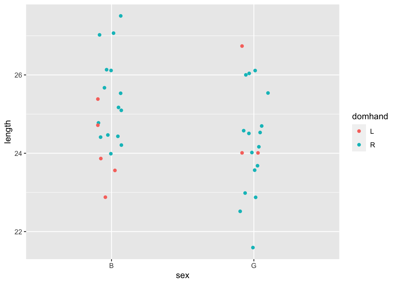
2. Graphics frame
A “graphics frame” defines how space and color are given meaning, each in terms of a variable.
We standardize on a single format for a frame:
- y-axis: the selected “response” variable.
- x-axis: a selected one of the explanatory variables.
- color: (optional) another selected one of the explanatory variables.
Any of these can be mapped to a numerical or a categorical variable, for example:
Graphical content
- The most common graphical content makes a mark for each specimen.
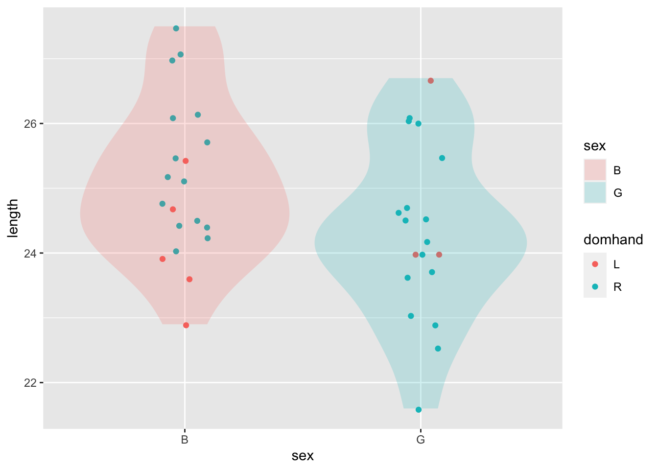
- Another (optional) form of graphical content reflects the data collectively: a violin.
- Still another (optional) form of graphical content also reflects the data collectively, but in terms of a regression model. (See below.)
Regression model
A regression model captures patterns in the data, typically the relationship between variables.
- Regression models always involve selecting, according to the modeler’s goals, a response variable which must always be numerical.
- There is also one or more explanatory variables. These can be either numerical or categorical.
- Regression models are constructed by “fitting” (or, equivalently, “training”) on a data frame. In addition to the data frame, a “model specification” must be provided which identifies the response variable and any explanatory variables.
Example:
my_model <- KidsFeet |> model_fit(length ~ sex + domhand)
model_plot(my_model)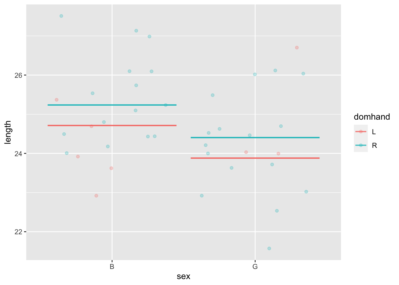
Important note: We don’t start with means and work toward regression. We start with regression.
Theoretical entities
In addition to the computational entities, there are several conceptual objects. These three show up in the second half of the Lessons.
4. Hypothesis
A statement that may or may not be true. In statistics, we are particularly interested in hypotheses that have some relevance to describing the world.
Note the “may or may not be true.” We emphasize this to move students away from the idea that a hypothesis should be something thought true or likely.
5. Probability model
Assignment of a number to each possible outcome. Across all outcomes, these add up to 1.
6. Likelihood model
Assignment of a number to one outcome under different conditions. Across all conditions, these do not have to add up to 1.
Note: The word “likelihood” does not show up in the index of most Stat 101 books. Distinguishing between “likelihood” and “probability” helps to emphasize the essential role of hypotheses. Making this distinction is a judgement call motivated by Einstein’s “Aber nicht einfacher.”
Examples of likelihoods:
- the p-value (included in all Stat 101 books): The hypothesis conditioned on is the Null.
- the power (not covered in detail in most Stat 101 courses). The hypothesis conditioned on is the Alternative.
- sensitivity in diagnostic tests. The hypothesis is that the person has the disease.
- specificity in diagnostic tests. They hypothesis is that the person does not have the disease.
In Bayesian inference, likelihoods are the means by which a prior probability is updated to a posterior probability. In the two-hypothesis setting, Bayes rule has an elegant form:
Posterior odds = Likelihood ratio \(\times\) prior odds