dagA <- dag_make(
  x ~ exo(1),
  y ~ 2 - 3*x + exo(2)
)Simulations with DAGs
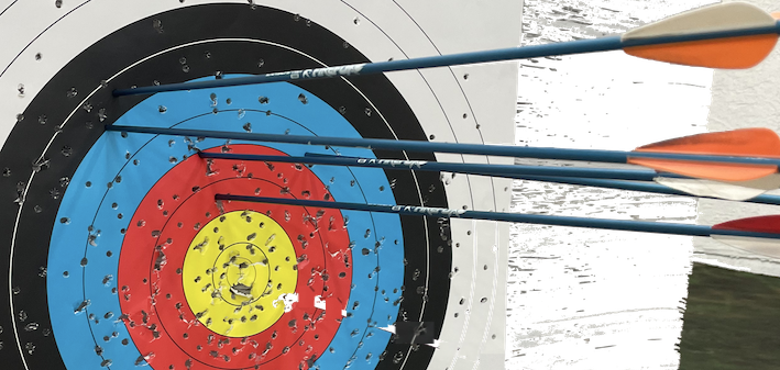
Most Stat 101 texts describe early on the distinction between accuracy and precision, often employing an archery metaphor: [Another pair of words—bias and variance are often used instead. “Bias” carries an inappropriate connotation of intentionality. Worse, “variance” also is our main measure of variation, which can be confusing when it is also about sampling variation.]
There are many topics in Stats 101 that focus on precision: confidence intervals, p-values, etc. Students learn how to quantify precision.
There is no similar emphasis on accuracy. We offer no methods to quantify inaccuracy. We do offer two prescriptions for avoiding inaccuracy:
- Random sampling
- Random assignment
Entirely outside the domain of the traditional Stats 101 course, there are routine techniques for correcting—adjusting for—inaccuracy. There are names for the source of one sort of inaccuracy: “model misspecification bias.” There are names for techniques to mitigate inaccuracy: “intent to treat” and “instrumental variables.” Just about every reputable news article about statistical results includes a phrase like “controlling for …” or “after adjusting for.” Polls that aim to be reputable never rely on an attempt to collect a random sample—it’s impossible. Instead, they use adjustment techniques such as stratification.
On the other hand, because methods for avoiding inaccuracy—except for random sampling and random assignment—are ignored by Stat 101 textbooks, many statistics instructors do no even know that such methods are a routine and accepted part of applied statistics. The result in a considerable disconnection between the graduates of Stat 101 and anyone who needs to use statistics in an applied way.
Important structural reasons for the failure of Stat 101 to take on accuracy-related methods include:
Stat 101 is largely a derivative of mathematical statistics. There is an important emphasis on unbiased statistics in mathematical statistics—think BLUE—but all that has already been dealt with by the nature of the statistics we teach to students: the mean, the standard deviation with \(n-1\) in the denominator, the degrees of freedom in the residual standard error. Mathematical statistics does not, however, have much to say about confounding, and nothing to say about the mechanisms of the physical world that motivate researchers to “control for ….”
Almost nothing in Stat 101 relates to having more than one explanatory variable. “Adjusting for …” is intrinsically a multi-variable process.
Stat 101 is allergic to any claim that understanding of causal mechanisms can come out of observational data. An estimate that is entirely misleading in terms of causality can nonetheless be unbiased as a pure description of probability relationships between variables.
My focus in this hour is on a small part of this: restoring a sensible balance between coverage of precision and accuracy in Stat 101. The lack of balance is a problem because it leads to a widely observed phenomenon: Stat 101 graduates—including science professionals—mistake precision for accuracy.
How to incorporate accuracy in Stat 101.
The type of inaccuracy that concerns me is that related to meaningful estimation of causal connections in the real world.
To demonstrate how statistical methods can produce accurate estimates, it’s necessary to compare the results from statistics to known facts.
There are setting in which there is practically universal consensus about facts in the real world. Example: smoking causes lung cancer. Data sets about this causal relationship—such as the Whickham data frame—are useful to demonstrate how failure to adjust for covariates can result in a misleading result. If there were 100 such settings where the facts are known, a compelling demonstration of how to avoid inaccuracy could be made. We can keep looking for them, and should. But to the extent to which the facts are not universally accepted and true, such demonstrations are (correctly) treated with skepticism.
To teach about accuracy, we need a way to create situations where the facts are demonstrably true. Two components are needed:
- The ability to collect arbitrary amounts of data. This lets us rule out matters of precision.
- Clear and evident demonstration of the mechanisms behind the data. When data analysis fail to replicate these known mechanisms, we can justifiably attribute the deviations to methodological artifact.
Both of these components are present in computer simulations of data generation.
In Lessons these simulations are provided by DAGs along with a mathematical formula for every hypothesized causal node.
DAGs (with simulation)
The DAGs used in Lessons are a hypothesis about causal connections made real by specifying formulas for each of the causal nodes.
We have students perform three operations on such DAGs:
- Sampling data from the simulation.
- Drawing the graph
- Examining the formulas for each node.
For instructors, I’ll start differently, with construction of a DAG. For example, here a DAG implementing a linear relationship between x and y.
Nonlinear relationships can also be stated. Linear ones are nice to start with because they enable linear regression to be used to estimate the functional form.
dag_draw(dagA)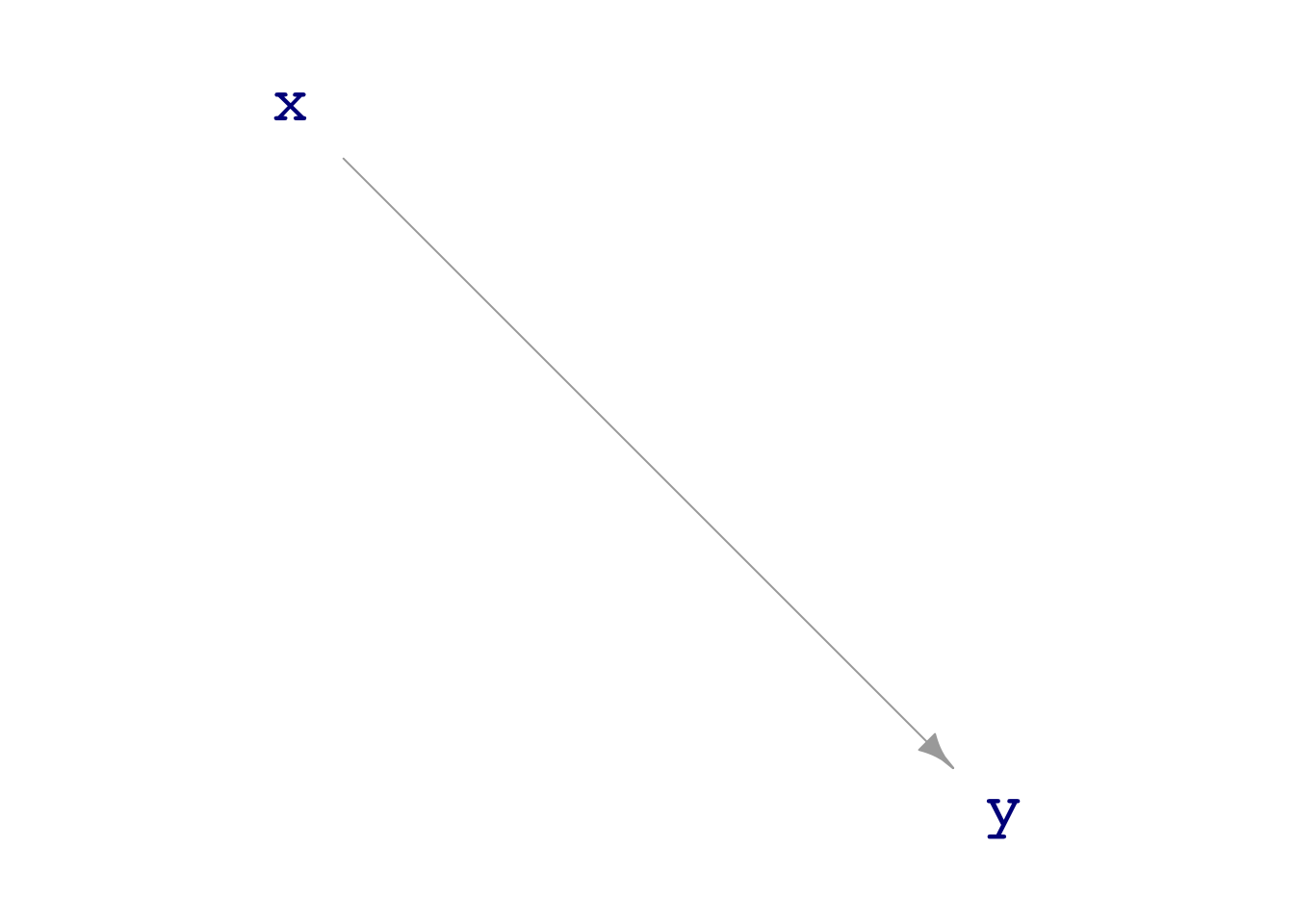
exo(s) corresponds to samples from a normal distribution with mean 1 and variance s-squared.
Generating a sample of size \(n=100\) is done with
Mysamp <- sample(dagA, size=100)This and the following tasks are pitched to instructors, who already know the statistical terminology and methods. I wouldn’t expect students to be able to address such questions until the end of the course. Even then, I would give them more guidance.
Your turn
Use the statistical techniques you know to demonstrate to your satisfaction the relationships implied in the dagA formulas.
Exercise 1
dag03 is a simple simulation of the relationship between (in Galton’s terms) a mid-parent and son. Show that there is regression to the mean.
dag_draw(dag03)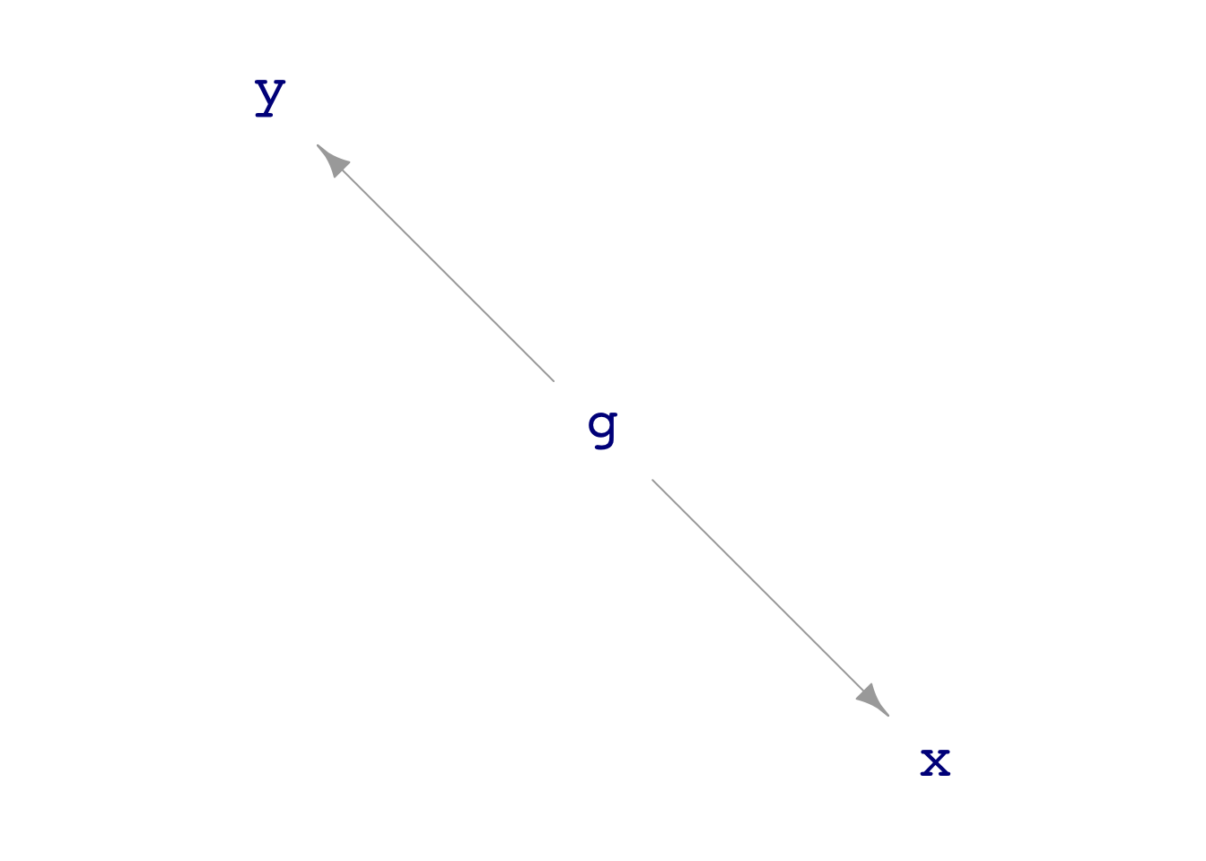
Exercise 2
dag02 has the causal topology called a “collider,” wherein y is caused by both x and a, but where there is no causal path between x and a.
Generate a sample from
dag02and show with the modela ~ xthat there is no non-trivial correlation betweenxanda. You can make the sample size as large as you want.Now construct the model
a ~ x + y. Is the coefficient onxnon-zero?
This is also known as “Berkson’s Paradox.” Jeff Witmer has some nice examples at section 15 of his paper on Stat 101
a and x is one where there is a node along the path where, placing water at that node will lead to it reaching both ends of the path. That’s not true in dag02.
Exercise 3
dag08 depicts a direct causal relationship between x and y that is confounded by c.
Look at the formulas for
dag08to read off the causal coefficient ofxony.Generate a sample (as big as you like) from
dag08and build the modely ~ x. Does the resulting coefficient onxmatch the coefficient from the DAG formulas?Same as (2), but use
cas a covariate. Is the match better or worse than in (2)?You can carry out a random assignment experiment with DAGs. To do so, you need to perform surgery on the DAG so that the values of the explanatory variable of interest,
x, are set by random assignment.dag_intervene()allows you to do such surgery, for instance:
my_experiment_dag <- dag_intervene(
  dag08,
  x ~ as.numeric(exo() > 0) )
Generate a sample of sufficient size from my_experiment_dag() and observe the coefficient on x in the model y ~ x. Does the coefficient match the causal formula for y?
dag_draw(dag08)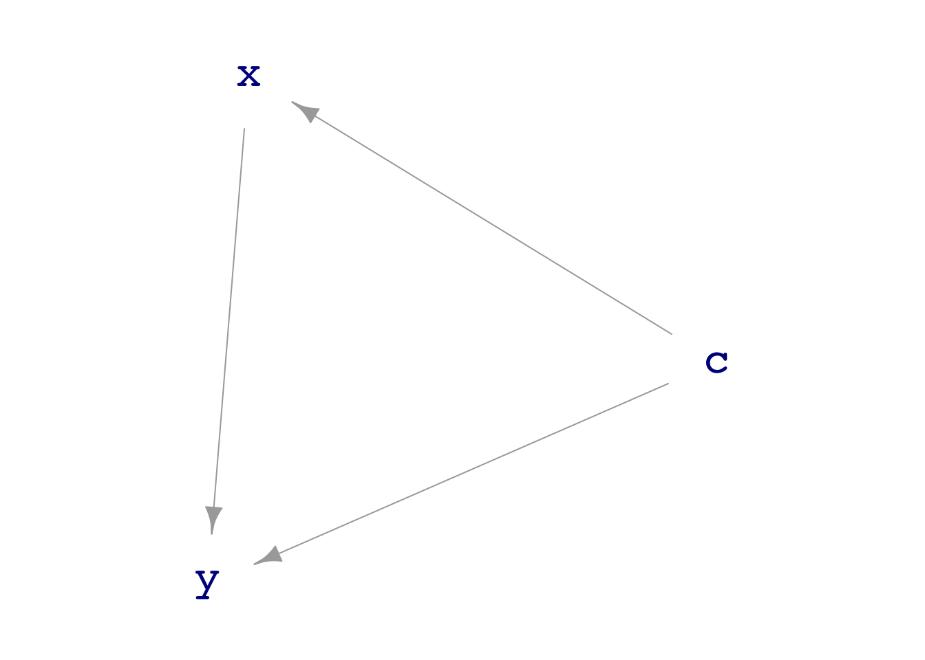
exo() draws from a standard normal distribution. exo() > 0 generates TRUE or FALSE completely at random. as.numeric() translates TRUE or FALSE into the numerical values 1 and 0 respectively.dag_draw(my_experiment_dag)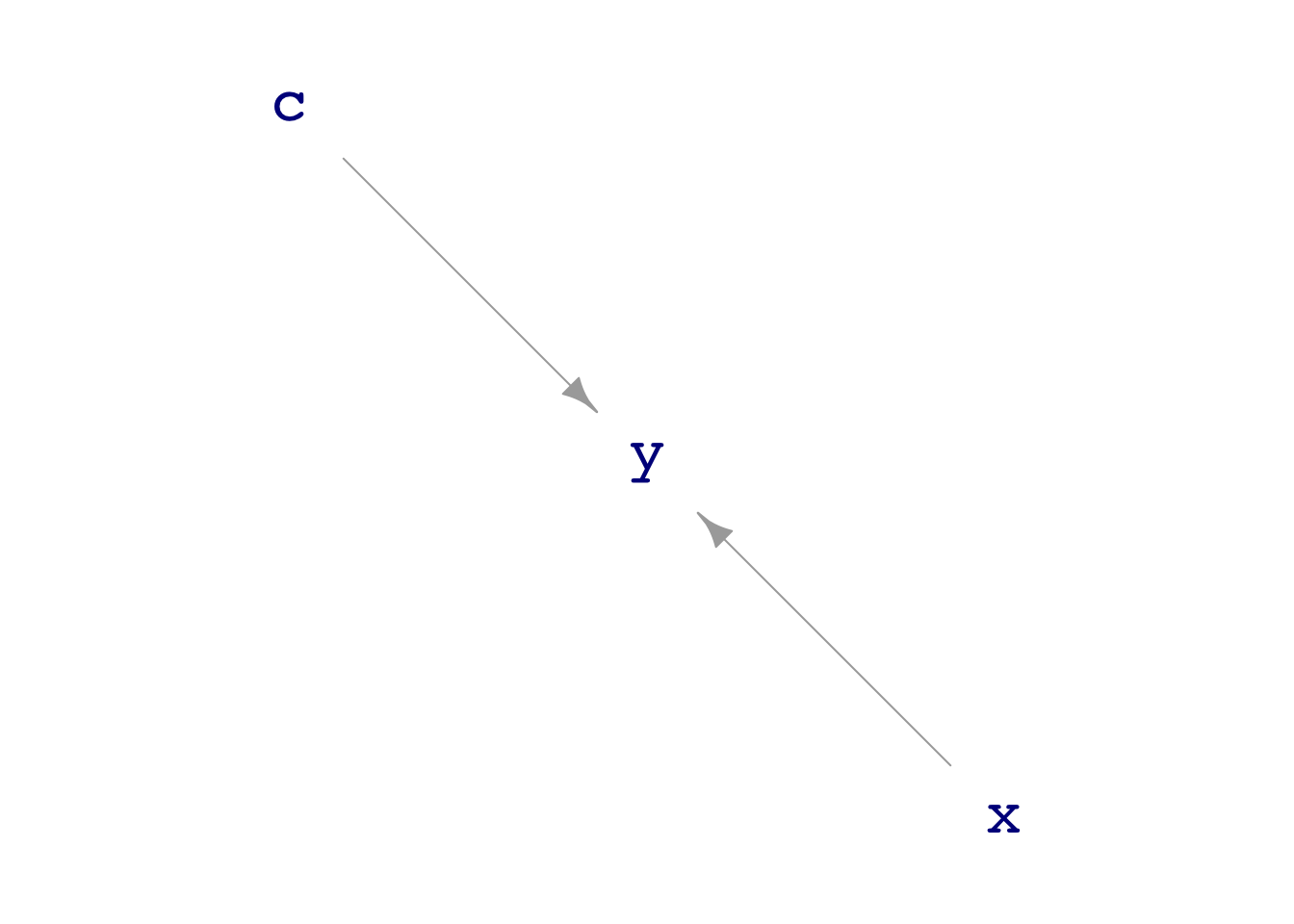
Verisimilitude
There is too much syntax in the construction of DAGs to expect that most students will be able to construct them. Nonetheless, a good class activity has groups of students construct causal hypotheses about real-world situations. The instructor can implement some of these (perhaps before the next class) and let students investigate the consequences of their hypotheses.
A quick starter guide:
- Remember to use TILDE expressions inside
dag_make(). - Numerical simulations are the simplest to construct.
- Use formulas with 1’s as coefficients, e.g.
y ~ x - c. - Use
exo()to add in exogenous noise. Each reference toexo()is an independent source of random numbers.
- Use formulas with 1’s as coefficients, e.g.
- There are also functions to generate bernouilli trials, categorical variables, etc. The documentation for the DAG system is minimal (see
?dag_make) and needs to be translated into a tutorial form.
Some of the DAGs provided by the {math300} package are simulations of hypotheses about events in the real world, e.g. dag_medical_interventions, dag_vaccine. With practice, an instructor can construct her own DAGs to represent causal hypotheses.
dag_flights is a simulation based on an Air Force Academy management exercise about the maintenence hours needed to support a morning and an afternoon training exercise with (nominally) ten planes.
There is a 6% chance that any one plane will need to abort on take-off and need repairs and a 12% chance that something on the plane might break while in flight and need repair on landing.
For the afternoon mission, an aborted flight from the morning will be ready with 0.67 probability. An inflight-breakdown is less likely, 0.4, to be ready for the afternoon flight.
Altogether, AM and PM give the number of planes that take of on the morning and the afternoon training mission.
Given the rates of breakage and the repair probabilities, what is the distribution of how many flights will take-off successfully each day? :::