Lesson 38: Worksheet

An important recommendation given by these Lessons is this:

Whenever possible, prefer confidence intervals to p-values.

This recommendation is consistent with the American Statistical Association’s “Statement on statistical significance and p-values”

“Statistical significance is not equivalent to scientific, human, or economic significance. Smaller p-values do not necessarily imply the presence of larger or more important effects, and larger p-values do not imply a lack of importance or even lack of effect. Any effect, no matter how tiny, can produce a small p-value if the sample size or measurement precision is high enough, and large effects may produce unimpressive p-values if the sample size is small or measurements are imprecise.” —From the ASA statement.

Confidence intervals, unlike p-values, convey clearly what is known about the size of an effect. For experts in the field of application, the effect size indicates the importance or utility of a relationship uncovered by statistical methodology. P-values do not do this even though they are widely misinterpreted as doing so.

Consider one widely used statistical practice, the use of a correlation coefficient as a measure of the strength of association between two variables, is often interpreted in terms of p-values. The correlation coefficient, r, is always between -1 and 1 and does not appear at first glance to be in the form of an effect size.

The point of this worksheet is to show that even a correlation coefficient can be translated into an effect size and a confidence interval.

Task 1. Use data wrangling and cor() to calculate the correlation coefficient between height and mother in the Galton data. Show that it doesn’t matter which order the variables appear in the argument to cor().

ANSWER

Galton |> summarize(r = cor(height, mother))

          r
1 0.2016549

Galton |> summarize(r = cor(mother, height))

          r
1 0.2016549

Task 2: Construct two models using Galton: (i) height ~ mother and (ii) mother ~ height. Show that the confidence intervals on the explanatory variable’s coefficient are not the same.

Note

lm(height ~ mother, data=Galton) |> conf_interval()

# A tibble: 2 × 4
  term          .lwr  .coef   .upr
  <chr>        <dbl>  <dbl>  <dbl>
1 (Intercept) 40.3   46.7   53.1  
2 mother       0.213  0.313  0.413

lm(mother ~ height, data=Galton) |> conf_interval()

# A tibble: 2 × 4
  term           .lwr  .coef   .upr
  <chr>         <dbl>  <dbl>  <dbl>
1 (Intercept) 52.7    55.4   58.2  
2 height       0.0885  0.130  0.171

The symmetry of the correlation coefficient contrasts with the lack of symmetry of the regression confidence intervals, leading many people to believe that a correlation coefficient is different in kind than a coefficient on an explanatory variable. However, this is not true. It is merely that the correlation coefficient involves a transformation of the variables.

Task 3. Using wrangling, add two new variables to Galton named H and M. These will be transformed versions of height and mother respectively. This type of transformation is called “standardization.”

H = (height - mean(height))/sd(height)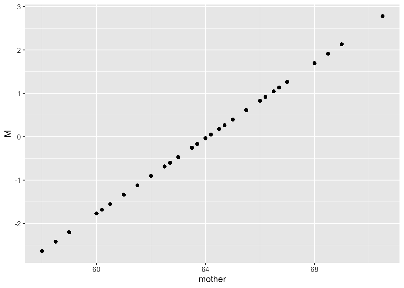
M = (mother - mean(mother))/sd(mother)

1. Plot H vs height and also M vs mother to show that the transformation is in the form of a straight-line function.

ANSWER

Galton <- Galton |> 
  mutate(H = (height - mean(height))/sd(height),
         M = (mother - mean(mother))/sd(mother))
ggplot(Galton, aes(x=height, y=H)) + geom_point()
ggplot(Galton, aes(x=mother, y=M)) + geom_point()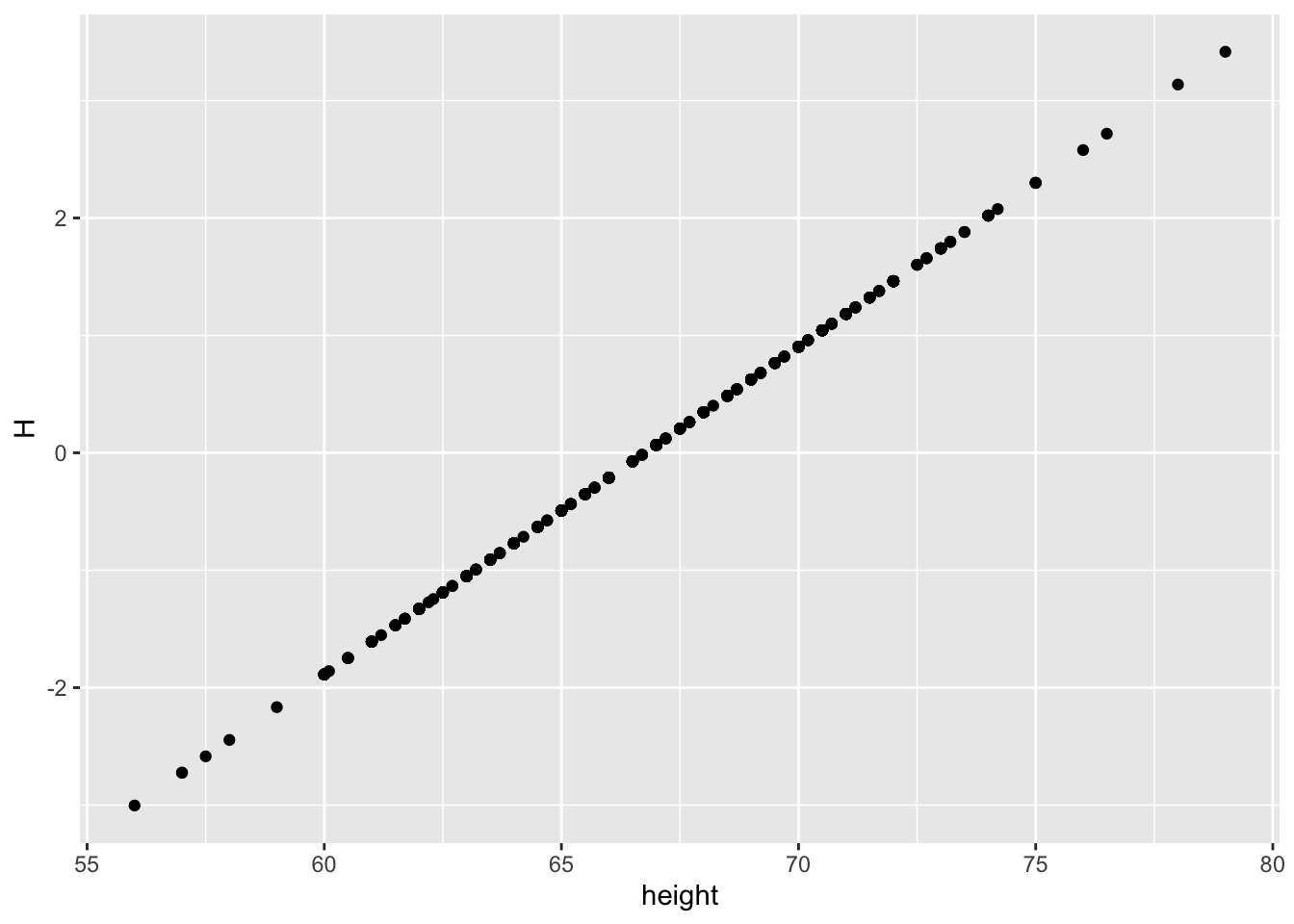

2. Find the means of both H and M and compare them to the means of height and mother. What’s special about H and M?

ANSWER

Galton |> 
  summarize(mH = mean(H), mM = mean(M), 
            mheight = mean(height), mmother = mean(mother)) 

            mH           mM  mheight  mmother
1 -6.74454e-16 8.554048e-16 66.76069 64.08441

The means of the standardized variables are zero. (A computer number like 6.7e-16 is effectively zero in this context; it differs from mathematical 0 because of computer round-off error.)

3. Compute the variance of both H and M and compare them to the variances of height and mother. What’s distinctive about H and M in this regard.

ANSWER

Galton |> summarize(vH=var(H), vM=var(M), vheight=var(height), vmother=var(mother))

  vH vM vheight  vmother
1  1  1 12.8373 5.322365

The variance of a standardized variable is 1.

4. Describe in words what the standardization transformation accomplishes?

ANSWER

A standardized variable has mean zero and variance one. If the original variable has units (e.g. height is in inches), the standardized variable is unitless.

Task 3: Fit the models H ~ M and M ~ H and find the confidence interval on the explanatory variable’s coefficient. The coefficients and confidence intervals are remarkable. Explain how.

ANSWER

lm(H ~ M, data=Galton) |> conf_interval()

# A tibble: 2 × 4
  term           .lwr     .coef   .upr
  <chr>         <dbl>     <dbl>  <dbl>
1 (Intercept) -0.0642 -6.58e-16 0.0642
2 M            0.137   2.02e- 1 0.266 

lm(M ~ H, data=Galton) |> conf_interval()

# A tibble: 2 × 4
  term           .lwr     .coef   .upr
  <chr>         <dbl>     <dbl>  <dbl>
1 (Intercept) -0.0642 -1.00e-15 0.0642
2 H            0.137   2.02e- 1 0.266 

The M coefficient is, in both models, exactly the same as the correlation coefficient. The intercept coefficient is zero (to within computer round-off error). The confidence intervals for the two models are exactly the same.

Task 4. The confidence interval on the standardized explanatory variable is describes the effect size of the standardized response variable with respect to the standard explanatory variable. Here is a graph showing the situation in terms of H vs M and the linear regression model:

mod1 <- lm(H ~ M, data=Galton)
model_plot(mod1) + coord_fixed() + labs(title="H vs M")
mod2 <- lm(M ~ H, data=Galton)
model_plot(mod2) + coord_fixed() + labs(title="M vs H")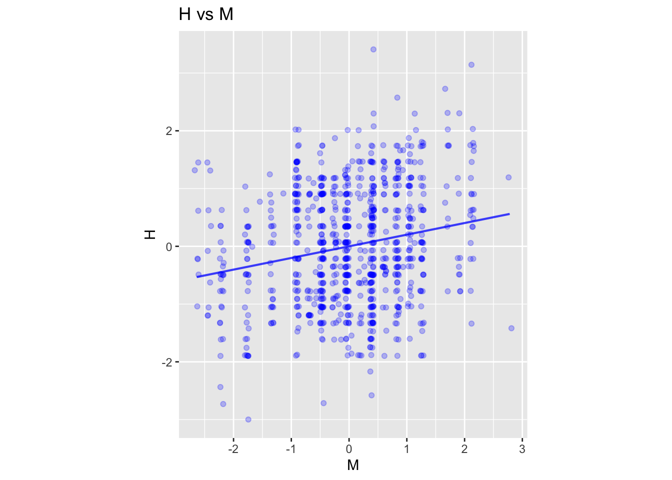

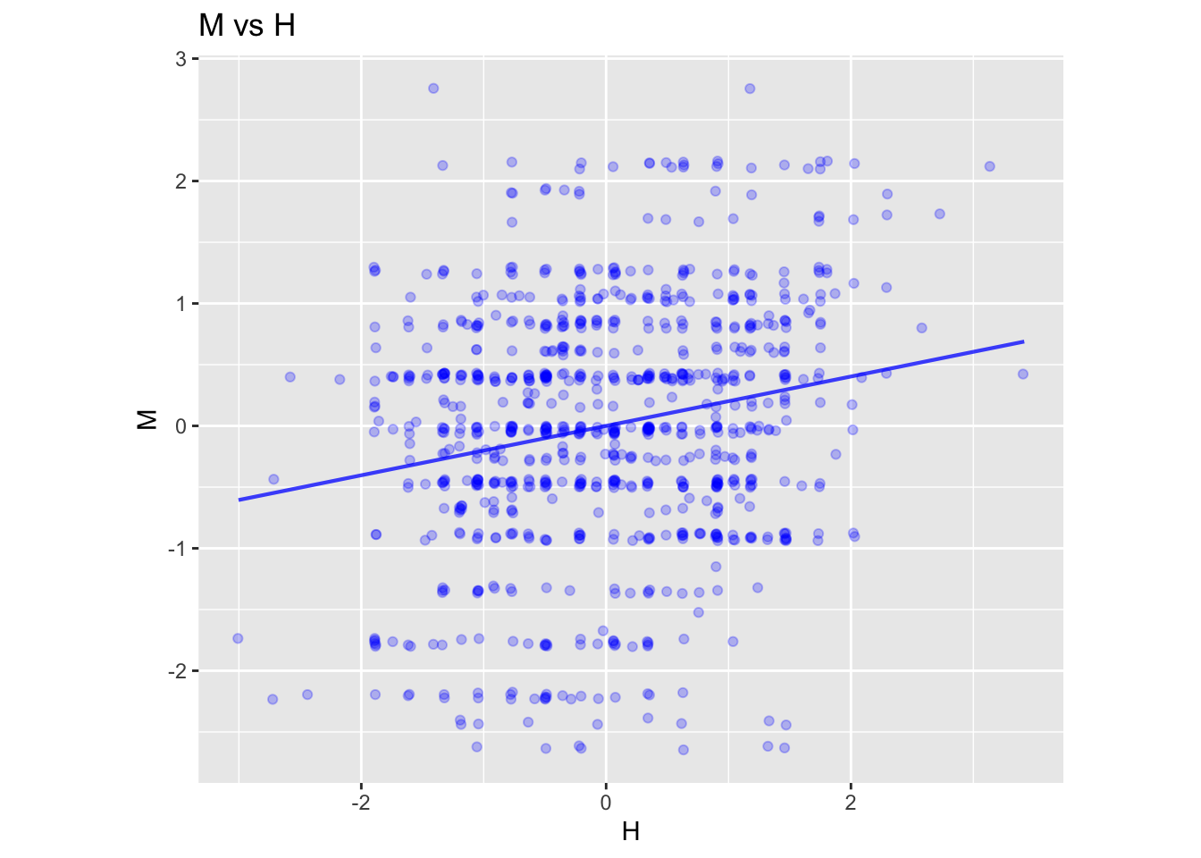
The quantities on the axes are denominated as “standard deviations.”

Question: From the graphs, estimate the effect size with respect to the explanatory variable.

ANSWER:

The slope of the line is the same in both graphs. A “run” of 2 units corresponds to a “rise” of about 0.4 units, so the slope is 0.4/2 = 0.2. This is exactly the meaning of the correlation coefficient: the effect size of one variable with respect to the other, both variables being given in units of standard deviations.

Task 5. The effect size is the expected change in the response variable for a 1 unit change in the explanatory variable. Since the effect size for H with respect to M (and the other way around, as well ) is 0.2016 we expect a 0.2016 standard deviation increase in the response for a 1.0 standard deviation increase in the explanatory variable. Stated another way, the slope of the regression line is

\(\text{slope} = 0.2016 \frac{\text{sd(response)}}{\text{sd(explanatory)}}\)

Calculate the standard deviation of both mother and height. Plug them in to the above formula for slope for each style of model, H ~ M and M ~ H. Where have you seen the resulting slopes before?

ANSWER

Galton |> summarize(sdmother = sd(mother), sdheight = sd(height))

  sdmother sdheight
1 2.307025 3.582918

0.2016*3.583 / 2.307 # for height ~ mother

[1] 0.3131048

0.2016*2.307 / 3.583 # for mother ~ height

[1] 0.129805

The slopes calculated here for the two different arrangements of the model are the same as the coefficients from the corresponding regression models, e.g. lm(height ~ mother, data=Galton)