Lesson 35: Worksheet

Author

Jane Doe

THIS WORKSHEET STILL IN DRAFT FORM. SKIP IT in favor of the in-class activity.

Build a model to stratify risk of CHD

mod1 <- glm(TenYearCHD ~ age + sex + BPMeds + diabetes, data=Framingham,
            family=binomial)

Simple threshold choice

Scores <- model_eval(mod1, interval="none")
ggplot(Scores, aes(x=as.factor(.response), y=.output)) + geom_jitter(alpha=0.1, width=0.2) +
  geom_violin(fill="blue", alpha=0.2)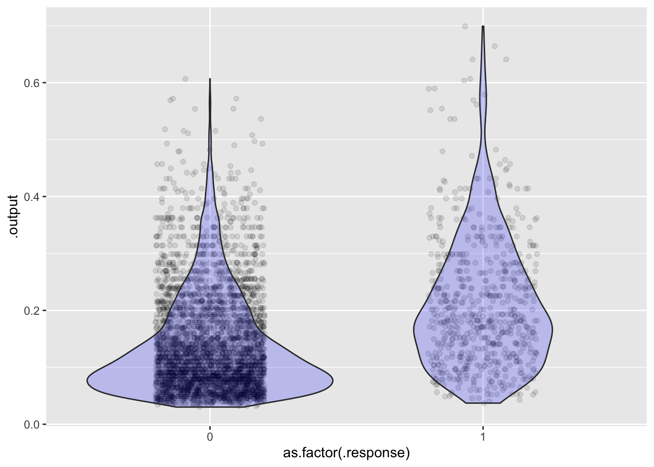

Pick a threshold

Let’s use 0.2

Construct the confusion matrix

And the sensitivity and specificity

Scores |> mutate(result=ifelse(.output > 0.2, "P", "N")) |>
  group_by(.response, result) |>
  tally() |>
  group_by(.response) |>
  mutate(frac = n/sum(n))

# A tibble: 4 × 4
# Groups:   .response [2]
  .response result     n  frac
      <dbl> <chr>  <int> <dbl>
1         0 N       2767 0.779
2         0 P        785 0.221
3         1 N        342 0.540
4         1 P        291 0.460

By changing the threshold, you can improve sensitivity at the cost of specificity and vice versa.

This isn’t a very good classifier, but let’s go with it.

Prevalence

In these training data, the prevalence of CHD is 15%.

Framingham |> summarize(prev = mean(TenYearCHD))

# A tibble: 1 × 1
   prev
  <dbl>
1 0.152

But let’s assume that the actual prevalence is 2%. Calculate the population false-positive and false-negative rates.