Clock_auction |> summarize(vprice = var(price), sd=sqrt(vprice))# A tibble: 1 × 2
vprice sd
<dbl> <dbl>
1 134203. 366.Signal and noise
Command patterns:
DF <- model_eval(MODEL)DF %>% summarize(NM = var(VAR) [, MORE] )model_eval(MODEL, VAR = VALUE [, MORE] )MODEL %>% R2()Every regression model involves a response variable, which Lessons in Statistical Thinking always plots on the vertical axis. Most of the regression models we will consider in these Lessons have one or two explanatory variables, although sometimes there will be more than two and sometimes none at all.
It is worth memorizing the forms of the tilde-expression specifications of the zero-, one-, and two-explanatory models, as well as their shapes. For this purpose, we’ll write the forms using five generic variable names. In practice, you will replace these generic names with specific names from the data frame of interest.
y — a quantitative response variable (which might be the result of a zero-one transformation).
x and z — quantitative explanatory variables
g and h — categorical explanatory variables.
| Model specification | Shape |
|---|---|
y ~ 1 |
A line with slope zero. |
y ~ x |
A line with possibly non-zero slope. |
y ~ g |
A value for each level of g. |
y ~ x + g |
Separate lines for each level of g, all with the same slope. |
y ~ x + z |
Parallel, evenly spaced lines. |
y ~ g + h |
For each level of g, a set of spaced values, one for each level of h. The h-spacing will be the same for every level of g. |
Note: It doesn’t matter what order the explanatory variables are given in. The name of the response variable is always on the left-hand side of the tilde expression.
Do Exercise 21.4.
By fitting a regression model, we divide the response variable into two components: a signal component and a noise component. The model specification tells what sort of signal to look for. For instance, the Clock_auction data frame records the sales price of antique grandfather clocks sold at auction. Presumably, the price reflects some feature of the clock itself as well as the market conditions. We have only the variables age and bidders to represent the the value of the clock and the market conditions.
Using lm() with the specification price ~ age directs the computer to look for a signal in the form of a straight-line relationship between age and price. The estimated noise is the difference between the response variable values (price) and the signal.
price? (Use the variance to measure variation.)Clock_auction |> summarize(vprice = var(price), sd=sqrt(vprice))# A tibble: 1 × 2
vprice sd
<dbl> <dbl>
1 134203. 366.Since the price is in dollars, the variance of price has units of “square dollars.” This is a unit that’s hard to get your head around. That’s why many people prefer the “standard deviation”, which is the square root of the variance.
price ~ age, then plot with model_plot(). Describe the pattern between price and age you see in the plot.mod1 <- lm(price ~ age, data=Clock_auction)
model_plot(mod1)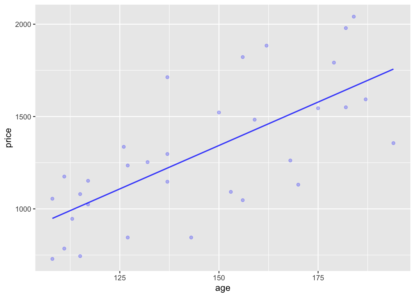
According to the model, price goes up with age. A 25 year increase in age corresponds to about a $200 increase in price.
Use model_eval() to find the model output for each clock for the model you constructed in (2).
.output? How does it compare to the variance of the response variable price?.resid. How much noise is there for price ~ age?.output, and the variance of the noise.Values <- model_eval(mod1)Using training data as input to model_eval().Values |> summarize(voutput = var(.output)) voutput
1 66352.26The variance of the model output (note the dot used in the name .output) is 66-thousand square dollars. (Why “square dollars?” Because the response variable is price which is in dollars. The model output always has the same units as the response variable. And the variance of a variable always has units that are the square of the variable’s units.) The variance of the price variable is about 134-thousand square dollars, so the model output has about half the variance of the response.
Values |> summarize(vresid = var(.resid)) vresid
1 67850.62The variance of the residuals is about 68-thousand square dollars. (The residuals always have the same units as the response variable.)
To show that the sum of the variances of the model output and residuals equals the variance of the response variable, just add them up and compare:
66352.26 + 67850.62[1] 134202.9The result exactly matches the variance of the price variable (calculated above).
R2() to summarize the model you constructed in (2). Demonstrate arithmetically the relationship between R2 and variances of the response variable and the model .output.mod1 |> R2() n k Rsquared F adjR2 p df.num df.denom
1 32 1 0.4944176 29.3375 0.4775648 5.914169e-06 1 30R2 is 0.49. This exactly matches the quotient of the variance of the model output divided by the variance of the response variable:
Values |> summarize(ratio = var(.output) / var(.response)) ratio
1 0.4944176.resid from part (3)?First, the value of 1 - R2, then the ratio of the variance of the residuals to the variance of the response variable:
1 - 0.4944176[1] 0.5055824Values |> summarize(ratio = var(.resid) / var(.response)) ratio
1 0.5055824dag10 has a simple structure, with nodes a through f each contributing to the value of y. Use sample() to generate a sample of size 1000. Using your sample, construct several models and calculate the R2 statistic.
y ~ 1.y ~ ay ~ by ~ a + bOur_sample <- sample(dag10, size=1000)
lm(y ~ 1, data=Our_sample) |> R2() n k Rsquared F adjR2 p df.num df.denom
1 1000 0 0 NaN 0 NaN 0 999lm(y ~ a, data=Our_sample) |> R2() n k Rsquared F adjR2 p df.num df.denom
1 1000 1 0.1163881 131.4552 0.1155028 0 1 998lm(y ~ b, data=Our_sample) |> R2() n k Rsquared F adjR2 p df.num df.denom
1 1000 1 0.2561369 343.6448 0.2553916 0 1 998lm(y ~ a + b, data=Our_sample) |> R2() n k Rsquared F adjR2 p df.num df.denom
1 1000 2 0.391591 320.8501 0.3903705 0 2 997The model y ~ 1 has R2=0 because the pseudo-variable 1 has zero variance and cannot “explain” any of the variance in the response variable y.
Model specifications like y ~ a are actually shorthand for y ~ 1 + a. So y ~ a has an additional explanatory variable in addition to the pseudo-variable 1. Whenever you add a new explanatory variable to an existing model specification, the R2 will increase (or, more precisely, cannot decrease).
y ~ a + b + c versus y ~ c + a + b.)Compare, for instance, y ~ a + b + c to y ~ c + a + b
lm(y ~ a + b + c, data=Our_sample) |> R2() n k Rsquared F adjR2 p df.num df.denom
1 1000 3 0.4293227 249.7649 0.4276038 0 3 996lm(y ~ c + a + b, data=Our_sample) |> R2() n k Rsquared F adjR2 p df.num df.denom
1 1000 3 0.4293227 249.7649 0.4276038 0 3 996The order of explanatory variables does not matter at all. It’s the collection that matters.
Write a sentence or two explaining what each of the following terms refers to.
Levels of a categorical variable. The values of a categorical variable are named. For instance, a household_pets variable would take on values like “cat,” “dog,” “turtle,” “parakeet,” …. The set of possible values for the categorical variable is called the “levels” of the variable.
Zero-one transformation. A means to translate a categorical variable with two levels into a quantitative variable. One of the levels is translated to the numerical value 1, the other to 0. The advantage of this particular scheme is that means or models where the zero-one variable is used for the response variable will have model outputs that can be interpreted as probabilities.
Model specification. When constructing a regression model, the modeler has to provide two different kinds of inputs: (1) a data frame for training the model, (2) a statement about which variable from the data frame to use as the response variable and which other variables to use as explanatory variables. This statement (2) is called the “model specification.”
Tilde expression. Tilde expressions are an element of the syntax (or “grammar”) of R. They always involve the tilde character (~) which has no other legitimate use in R. Any valid R expression can be used on the right-side of tilde. The left side (if present, as will be the case when used with lm()) can also be any valid R expression. The most prominant role for tilde expressions in Math 300Z is to hold the model specification for use by lm(). In this use, the response variable’s name always goes on the left side of the tilde. Explanatory variable names go on the right side, usually separated by + as punctuation.
For the computer-science oriented …. Tilde expressions are a way to represent symbolic expressions such as fragments of code. In ordinary use, R tries to evaluate every code fragment, replacing names with their values and invoking any functions used. Symbolic expressions are taken literally as a code fragment, without any evaluation. This is valuable as a means to pass code fragments to a function which can then parse or otherwise evaluate the fragment in a particular context.
Here’s a model of human height versus age based on the NHANES::NHANES data frame. (The package NHANES has the data frame which itself is called NHANES, so the full name is NHANES::NHANES.)
mod1 <- lm(Height ~ Age, data = NHANES::NHANES)
model_plot(mod1, data_alpha=0.05)
Warning: Removed 353 rows containing missing values (`geom_point()`).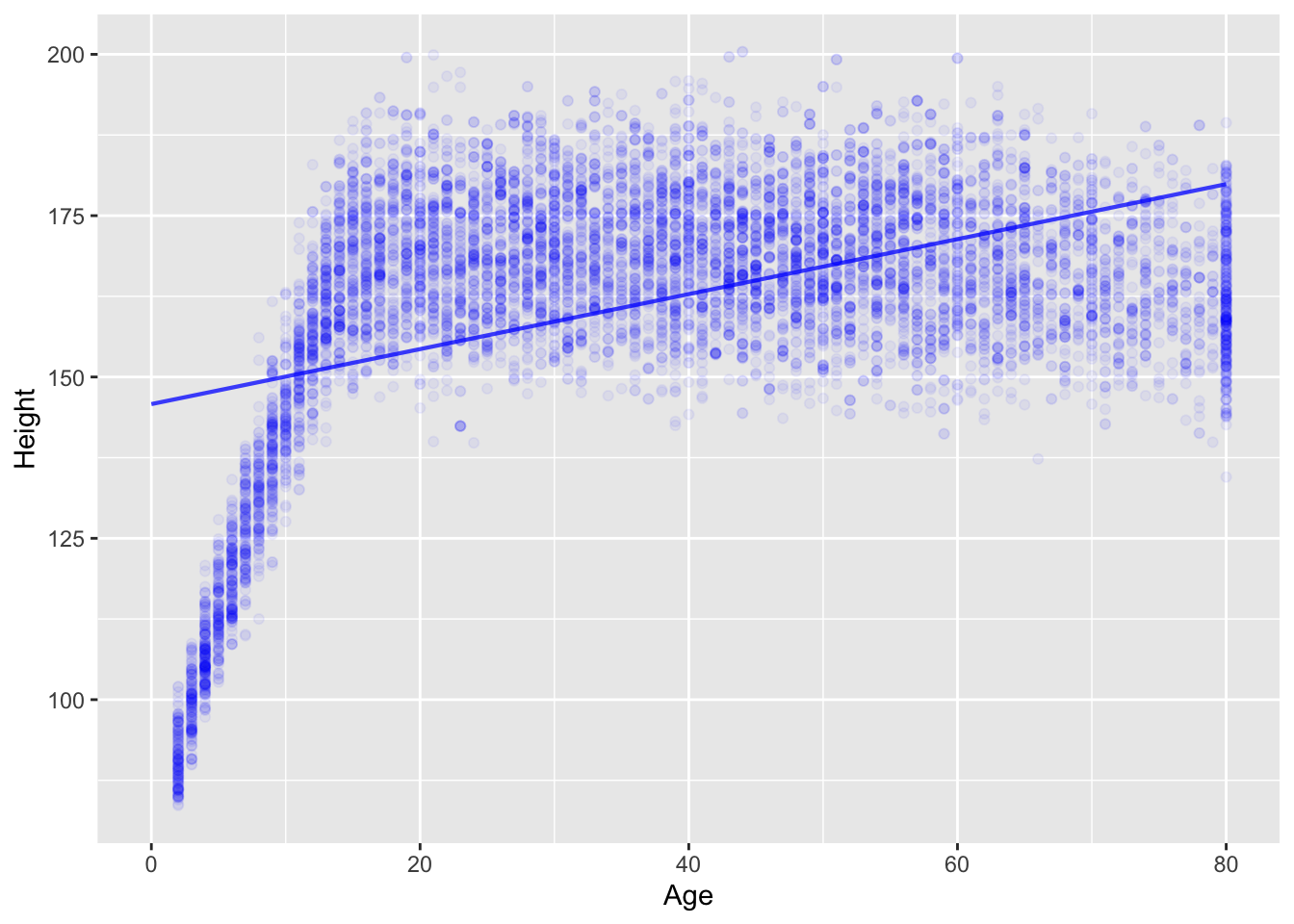
Age and Height? Explain using simple biological terms what the problem is with the straight-line model.Humans and other animals grow in a non-linear manner: rapid growth during gestation, infancy, and youth and comparative stasis later in life. With a model specification like Height ~ Age, lm() will look for a purely linear function, as in the straight line in the above graphic. The linear function doesn’t capture the age-dependent growth rate (fast during youth, slow or nil in adulthood), since a straight line has the same slope at all values of the explanatory variable.
One of the signs of the ill-fit of a linear model is that the response values tend to be cluster mostly below or mostly above the line for different regions of the explanatory variable. For instance, in the graph above, for ages younger than 10, the height values are systematically below the straight-line function.
There are several modeling techniques for constructing models that are more flexible than a straight line. We won’t be using them in Math 300, but we want to point out that they exist. Try this one:
mod2 <- lm(Height ~ splines::ns(Age,5) * Gender, data = NHANES::NHANES)
model_plot(mod2, data_alpha=0.05)
Warning: Ignoring unknown aesthetics: fillWarning: Removed 353 rows containing missing values (`geom_point()`).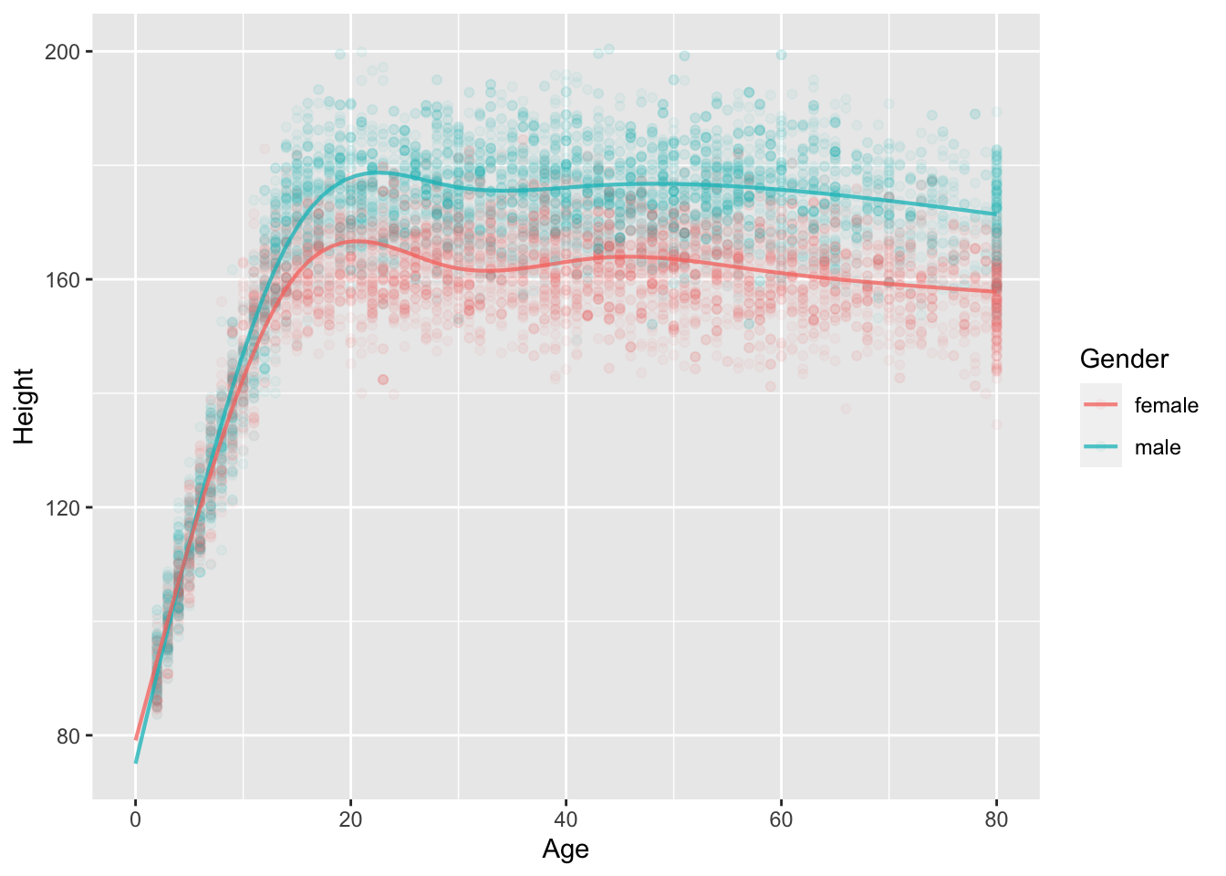
mod1 |> R2() n k Rsquared F adjR2 p df.num df.denom
1 9647 1 0.2117647 2591.193 0.2116829 0 1 9645mod2 |> R2() n k Rsquared F adjR2 p df.num df.denom
1 9647 11 0.8720171 5968.044 0.871871 0 11 9635The R2 for the rigid, straight-line model is substantially lower than for the more flexible, curvy model. Another way of saying this is that the curvy model stays closer (on average) to the data than the straight-line model.
An important theoretical question in statistical modeling is when to prefer a curvy model to a straight-line model. We haven’t yet encountered the statistical concepts that address this question.