Teaching notes, Lesson 24

Math300Z

Here are some fundamentals:

1. Every one of our modeling tasks starts with two things:
   1. A data frame (which might be from the real world or from our hypothetical world of DAGs)
   2. A model specification which names what variable is to be the response (or “output”) of our model and which variables are in the explanatory role.
      • We denote with a tilde expression: response ~ explan1 + explain2 + ...
      • There might be multiple explanatory variable, or just a single one, or even none, which we denote with 1.
2. We turn the (a) data frame and (b) model specification into a set of coefficients.
   1. We are using lm() as the engine for turning (a) and (b) into coefficients.
   2. This is a completely automatic process. It will give the same results in any software package, but setting up the calculation may be tedious and error-prone in some packages.

Galton |> model_train(height ~ mother + father + sex)

Call:
lm(formula = tilde, data = data)

Coefficients:
(Intercept)       mother       father         sexM  
    15.3448       0.3215       0.4060       5.2260  

Regression modeling in Excel

1. Install the Analysis Toolpack
2. If any of the explanatory variables are categorical, convert them to dummy variables. (Move insert column before sex, call it sexM, and give formula =(E2="M") + 0.)
3. Press “Data Analysis” in menu bar.

Output is placed in new sheet. In the Galton example, the coefficients are only slightly wrong, pretty good for Excel. (The linear algebra routines in the “Analysis Toolpack” are not state of the art. Probably they use “pseudo-inverses.”)

3. There are a variety of summaries of models available. Almost always, we will use conf_interval() or R2().

Galton |> 
  model_train(height ~ mother + father + sex) |>
  conf_interval()

# A tibble: 4 × 4
  term         .lwr  .coef   .upr
  <chr>       <dbl>  <dbl>  <dbl>
1 (Intercept) 9.95  15.3   20.7  
2 mother      0.260  0.321  0.383
3 father      0.349  0.406  0.463
4 sexM        4.94   5.23   5.51 

5. The confidence tells you the precision of the numerical measurement of the coefficient. If two coefficients have confidence intervals that overlap (like mother and father here) you don’t have a good basis to claim that they are different.

Why so much interest in coefficients?

1. An important statistical task (in some situations) is to detect whether there is some connection between an explanatory variable and the response variable. This often amounts to asking whether a coefficient is zero. More precisely, asking whether the confidence interval includes zero.

2. Mathematical tradition. There are other ways to present the same information. But people with a good head for mathematics find the coefficients easy to interpret … until the models become complicated.

3. Here’s a way to plot out the Galton model:

gmodel <- Galton |> 
  model_train(height ~ mother + father + sex)
model_plot(gmodel)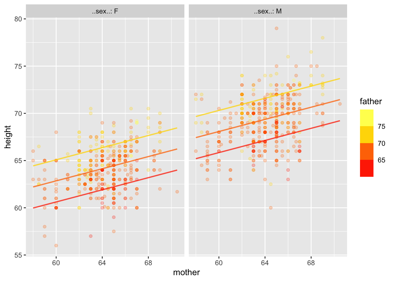

4. We can also show sampling variability graphically, although the plots can be hard to interpret.

model_plot(gmodel, interval="confidence")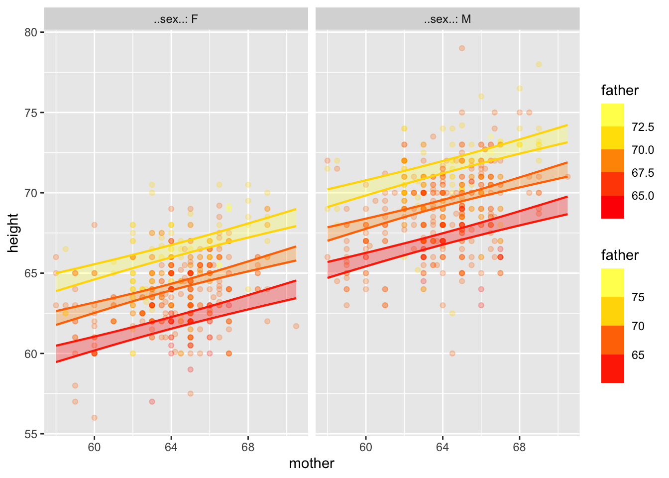

5. Another important type of statistical questions involves intervention: If we change the value of an input to the model, how much will the output change?

model_eval(gmodel, mother=c(60,65), father=65, sex="F")

  mother father sex  .output     .lwr     .upr
1     60     65   F 61.02304 56.77622 65.26986
2     65     65   F 62.63052 58.38981 66.87122

This is called an “effect size.” From the above table, we can calculate the effect size with respect to mother.

Effect size

1. An effect size (for numerical variables) is a partial derivative of the model function.

2. An effect size (for categorical variables) is a partial difference.

3. Whether a model’s effect size says what would happen in the real world if we changed a model input depends on whether we have captured causal connections properly with our model.

We can’t change the explanatory variables in a meaningful way in human height, but suppose the experiment were to make kindergarten class sizes smaller and look for the effect on later student achievement.

4. Calculate an effect size: use model_eval() changing one variable at a time.

5. Calculating confidence interval on effect size: Involves a lot of accounting, except in the simplest cases.

6. Units of effect size.

   • Quantitative variable: [response]/[explanatory] a rate (a.k.a slope)
   • Categorical variable: [response]

Why always + in model specifications

This is just for us, to make model interpretation easier.

With + models, the coefficient is always the same as the effect size.

But not generally. Examples with Galton data

mod1 <- lm(height ~ mother*father*sex, data=Galton)
model_plot(mod1)

Warning: Ignoring unknown aesthetics: fill

Notice that the lines aren’t parallel. We can also do curvy functions.

library(splines)
mod2 <- lm(height ~ ns(mother,2)*ns(father,2)*sex, data=Galton)
model_plot(mod2)

Warning: Ignoring unknown aesthetics: fill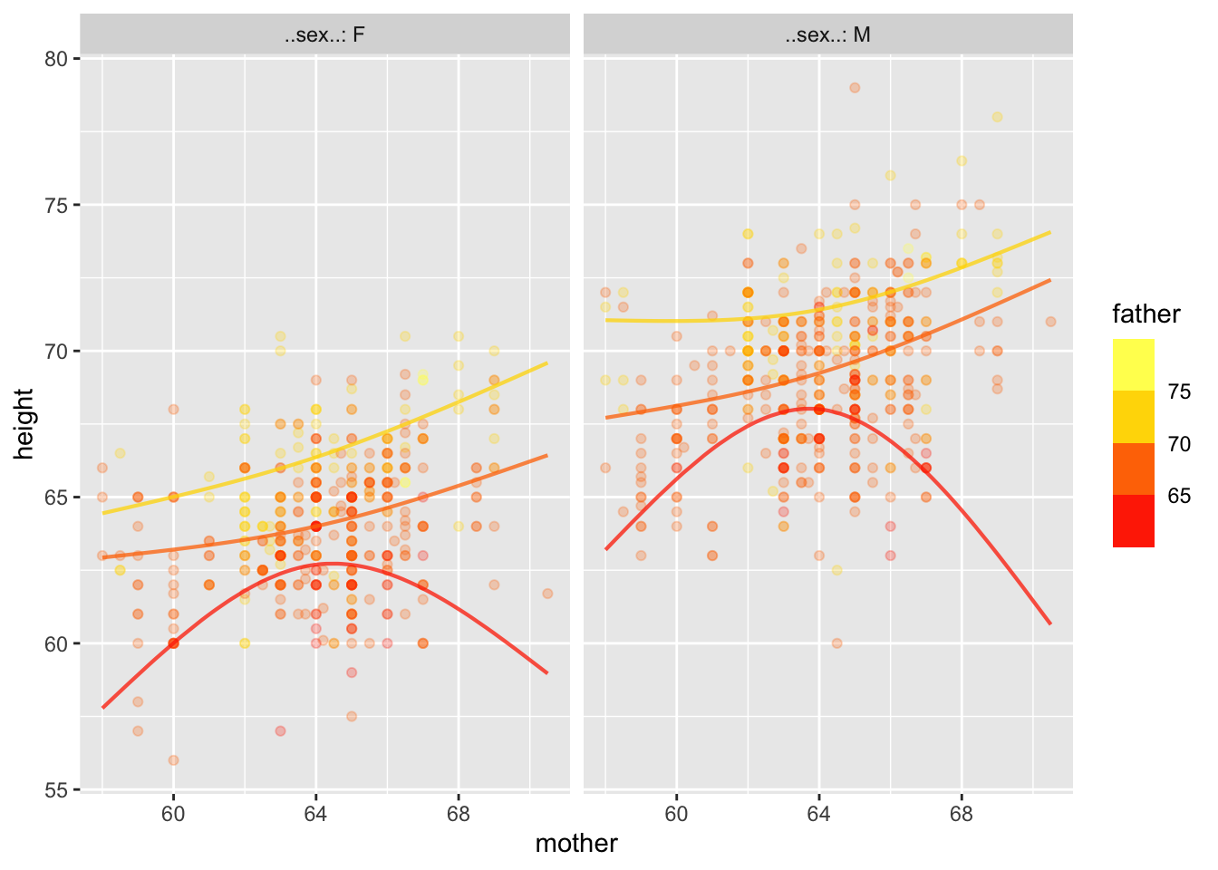

Might the curviness or non-parallel nature of the lines just be a matter of sampling variation?

model_plot(mod1, interval="confidence")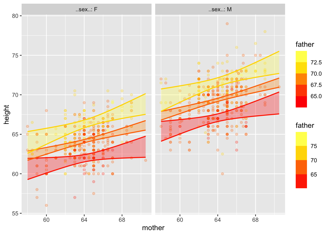

model_plot(mod2, interval="confidence")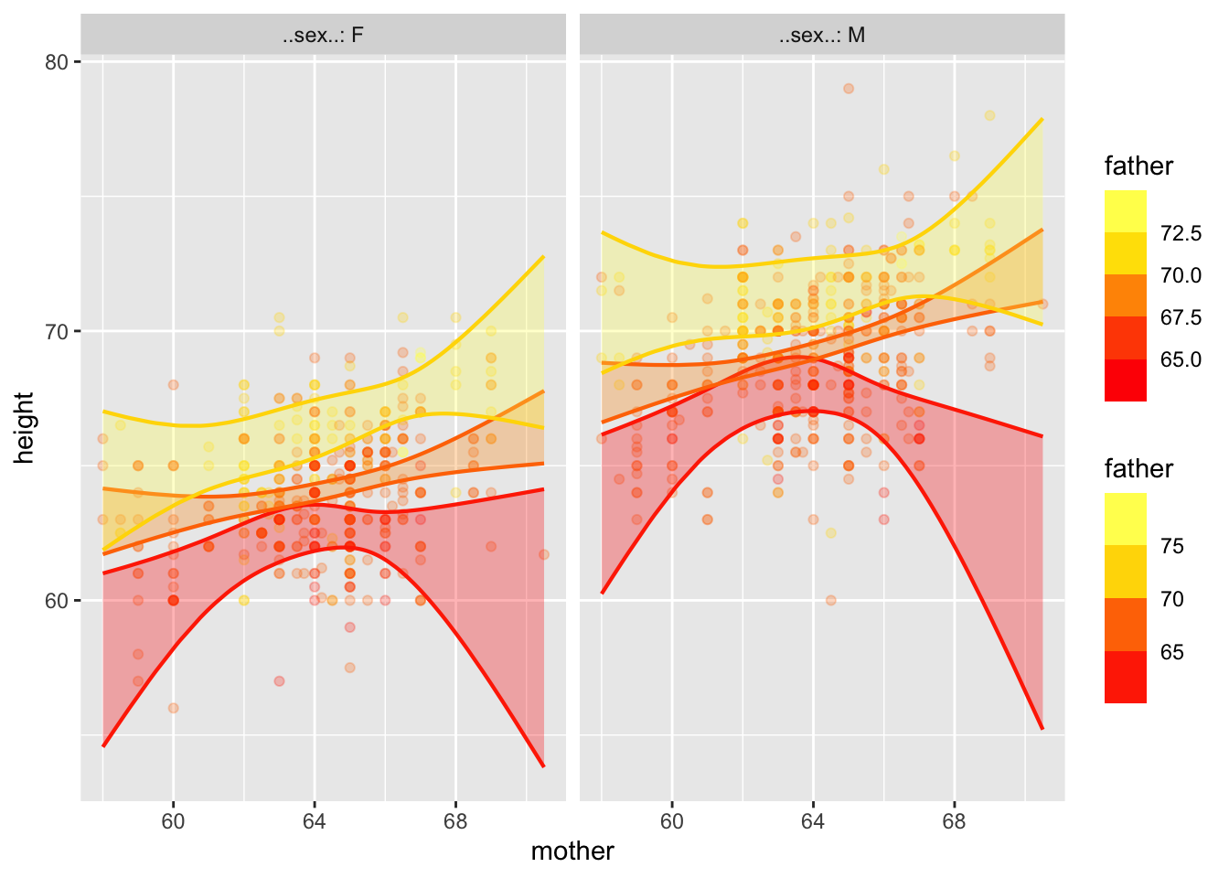

All the information for the confidence bands is contained in the coefficients (and residuals), but good luck figuring it out!

mod2 |> conf_interval()

# A tibble: 18 × 4
   term                                  .lwr   .coef  .upr
   <chr>                                <dbl>   <dbl> <dbl>
 1 (Intercept)                         50.1    55.4   60.7 
 2 ns(mother, 2)1                       1.01   10.7   20.5 
 3 ns(mother, 2)2                     -13.0    -4.36   4.31
 4 ns(father, 2)1                       4.97   15.4   25.9 
 5 ns(father, 2)2                      -0.486   4.98  10.5 
 6 sexM                                -1.19    6.00  13.2 
 7 ns(mother, 2)1:ns(father, 2)1      -32.1   -12.8    6.55
 8 ns(mother, 2)2:ns(father, 2)1       -1.03   15.1   31.3 
 9 ns(mother, 2)1:ns(father, 2)2       -8.41    2.27  12.9 
10 ns(mother, 2)2:ns(father, 2)2       -3.90    4.43  12.8 
11 ns(mother, 2)1:sexM                -17.3    -3.92   9.43
12 ns(mother, 2)2:sexM                -19.7    -6.97   5.72
13 ns(father, 2)1:sexM                -15.0    -0.854 13.3 
14 ns(father, 2)2:sexM                 -4.29    3.48  11.3 
15 ns(mother, 2)1:ns(father, 2)1:sexM -20.2     6.10  32.4 
16 ns(mother, 2)2:ns(father, 2)1:sexM -10.1    13.2   36.5 
17 ns(mother, 2)1:ns(father, 2)2:sexM -23.4    -8.08   7.25
18 ns(mother, 2)2:ns(father, 2)2:sexM -15.8    -2.90   9.97

Statisticians keep in mind this folk wisdom:

If you try to capture too much detail in the relationship, you won’t capture anything.

Notice that all but three of the terms have confidence intervals that include zero.