Review from Lesson 21
- A DAG (directed acyclic graph) is a way of representing a hypothesis or belief or possibility to be considered of the causal connections among variables.
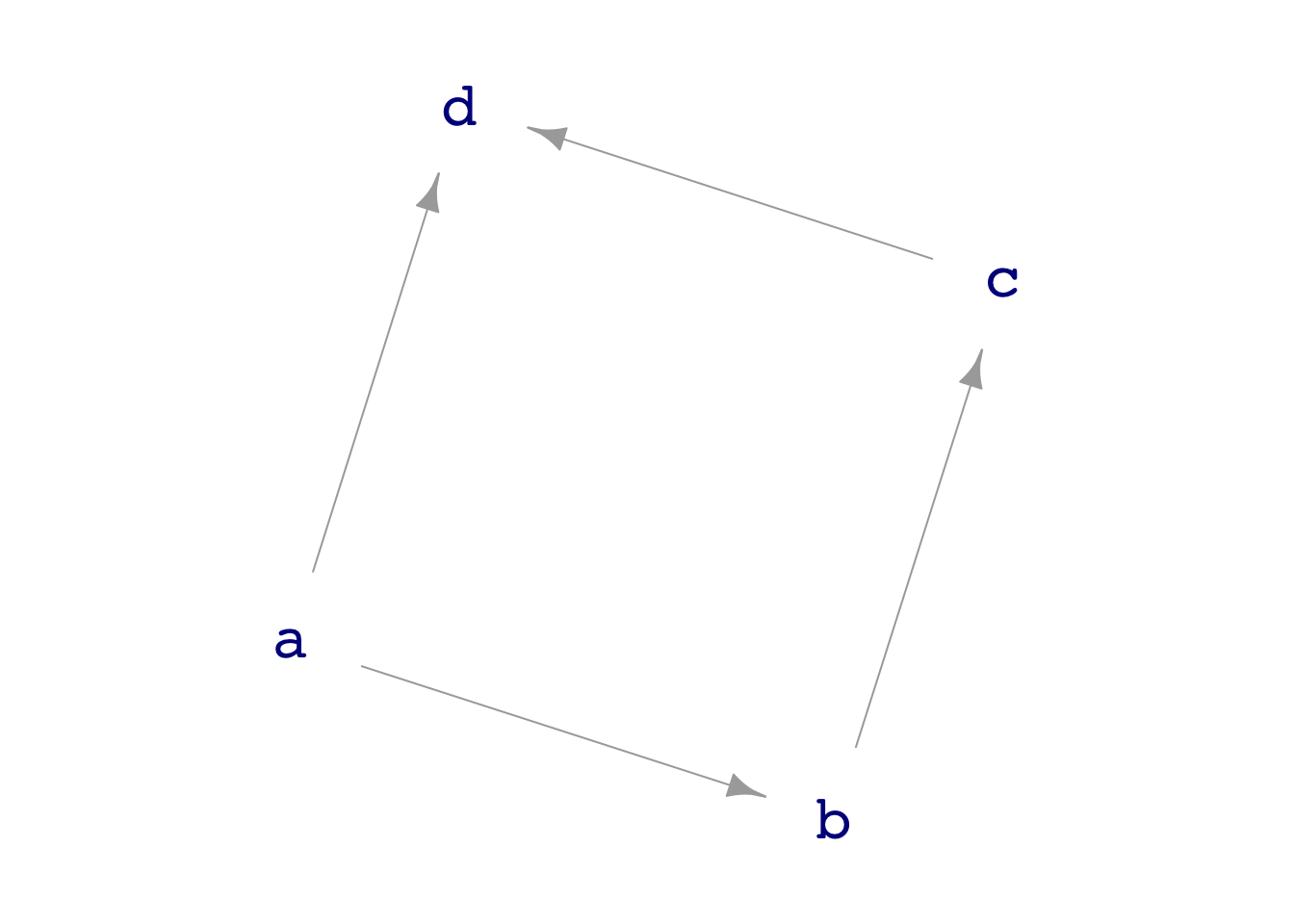
dag06, to use as an example.- DAGs consist of **nodes**---`a`, `b`, `c`, and `d` above, each representing a variable.
- Any pair of nodes can be connected (or not!) by a **directed edge**. The edge means that the two variables are causally connected. The one-way flow of influence from one variable to the other is indicated by the direction.
- The **A** in D**A**G stands for "acyclic," meaning that there are no loops (cycles) in the flow.We will use DAGs for three purposes:
- To encapsulate hypotheses about causal connections in a variety of real-world settings.
- As a means to reason about which covariates should and should not be included in a model. (Lesson 30)
- To generate data from a source whose mechanism is exactly known. This will allow us to learn how and how much we can learn from data. We can then carry these lessons to real situations where the mechanism is only hypothetically known.
The software for our use of DAGs is built in to the
{math300}package. This includes:- About a dozen different DAGs providing examples of different sorts of causal connection. This includes those named
dag01throughdag12, which are meant to be schematic (abstract). Other built-in DAGs encode hypotheses about causal connections in real-world systems. sample(dag01, size=10)generates data.dag_draw(dag01)draws a picture of the graph.print(dag01)shows the formulas used in the generation of simulated data.- In Lesson 32 (about experimentation) you will see how to change a DAG using
dag_intervene(). dag_make(..formulas..)creates a DAG, but you won’t have much occasion to use it.
- About a dozen different DAGs providing examples of different sorts of causal connection. This includes those named
Lesson 22
- Often, the data we have at hand is a sample of specimens from a much larger population of objects (called a “population”). We store the sample’s observations in a data frame.
- Even when the data are a census, we often analyze them as if they are a sample from a population.
- A statistical point of view is that the data in our data frame are merely one sample collected at random from the population. Consequently, we imagine for the purpose of constructing many statistical methods, that there are infinitely many other samples that are equivalent to the one we have but which just happened not to be selected.
- Sample statistics are numbers that we calculate from our sample. For us in Math 300Z, such statistics will typically be coefficients from a model (but we will also use some other sample statistics).
- Owing to the randomness involved in collecting our sample, we regard any sample statistic as a random draw from a population of sample statistics that could have been computed on other samples (as in (3)). That is, every sample statistic is a combination of “signal” and “noise.”
- Since our sample statistic includes noise, it is appropriate to quantify how much noise there is. Knowing this can, for example, enable us to decide whether two different samples come from different populations or not.