Review from Lesson 20
dag06, to use as an example.DAGs (“directed acyclic graphs”) have three properties, all of which are essential for representing causality.
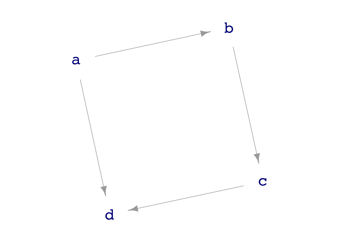
- They are “graphs” in the technical vocabulary of mathematics. That is, they consist of nodes and edges. Each edge connects two (and only two) of the nodes. In Figure 1 there are four nodes, labeled
a,b,c, andd. Coincidentally, there are also four edges, one of which isc\(\longrightarrow\)d. - Every edge is directed, that is, it points from a source node to a target node. Think of the directed edge as if it were a pipe carrying causal “fluid” from the source to the target. All the pipes in a graph are one-way only. In Figure 1 each of the edges is an arrow. The edge
a\(\longrightarrow\)bmeans that causal “fluid” can flow fromatob, but not frombtoa. - There are no loops in the fluid flow (that is, there are no “cycles” of flow). In the name DAG, this is the meaning of the A: “acyclic,” meaning “no cycles.”
- They are “graphs” in the technical vocabulary of mathematics. That is, they consist of nodes and edges. Each edge connects two (and only two) of the nodes. In Figure 1 there are four nodes, labeled
Starting in Lesson 30, we will get into the ways to use DAGs in order to select explanatory variables that produce a model that is a faithful representation of the causal flows.
For the next few lessons, we will use DAGs for another purpose: to simulate data and make it easy to conduct random trials.
Other than for teaching purposes (as in (3)), the role of DAGs in statistics and data analysis is to encode hypotheses about how elements of a system might be connected. Usually, you work with DAGs that reflect your and your colleague’s beliefs about how things are connected in the real world. Of course, believing a hypothesis does not make it true. Think of a DAG as a piece of fiction. Sometimes fiction is close to real life, and sometimes not. Both situations have their purposes for story-telling.
Lesson 21
It is helpful to think of any response variable as a combination of “signal” and “noise.” The signal reflects how the explanatory variables are related to the response. The noise is the unexplained part of the response variable. More precisely, the “noise” is that part that we do not care to explain in terms of relationships to other variables.
The idea that there is always noise in the response variable allows us to train models that do not go through every (or even any) data point. This enables us to claim that simple shapes of models can be good representations of relationships among variables.
In Math 300Z, with few exceptions we will work with models that have one or two explanatory variables. A nicer feature of such models is that we can draw a graphic of the model using just two or three aesthetics.
aes(y= ), the vertical axis: always will be assigned to the response variable. (This is a Math 300Z convention, and a good one, but not universal.)aes(x= ), the horizontal axis: the first explanatory variable will be assigned to this.aes(color= )if there is a second explanatory variable, it will be assigned to color.
The
model_plot()function will take care of all this assignment of variables to aesthetics.Since explanatory variables can be either categorical or quantitative, there are only a handful of model shapes we need to deal with. (The response variable is always quantitative.) These are enumerated in the Instructor’s notes for Lesson 21.
An excellent type of exam question would show you the graph of a model and ask you to identify whether there is one or two explanatory variables, and what type(s) it (they) are: quantitative or categorical.
There is also a role in statistics for models that have zero explanatory variables. The tilde expression for such models (letting
ybe the response variable) isy ~ 1. We have not yet discussed what the use is of such models.The data used to build a regression model is called the training data. It is a data frame containing both the response variable and any explanatory variables. Once a model is built, we often run the rows of the training data through the model function. Doing this divides the response variable values into two components:
- The signal, which is the model function output for each row of the training data. We call this the “model value.”
- The noise, which for each row of the training data is the difference between the value of the response variable (the “response value”) and the “model value.” This difference—one for each row of the training data—is called the “residual”.
Remember this simple relationship:
response value = model value + residual
- Often we will need to measure how big these three things are. We use the variance as the measure of “how big.” The variance is only one of many possible ways to quantify “how big.” But it has the great advantage that
var(response value) = var(model value) + var(residual)