Bayesian updating for self-driving cars

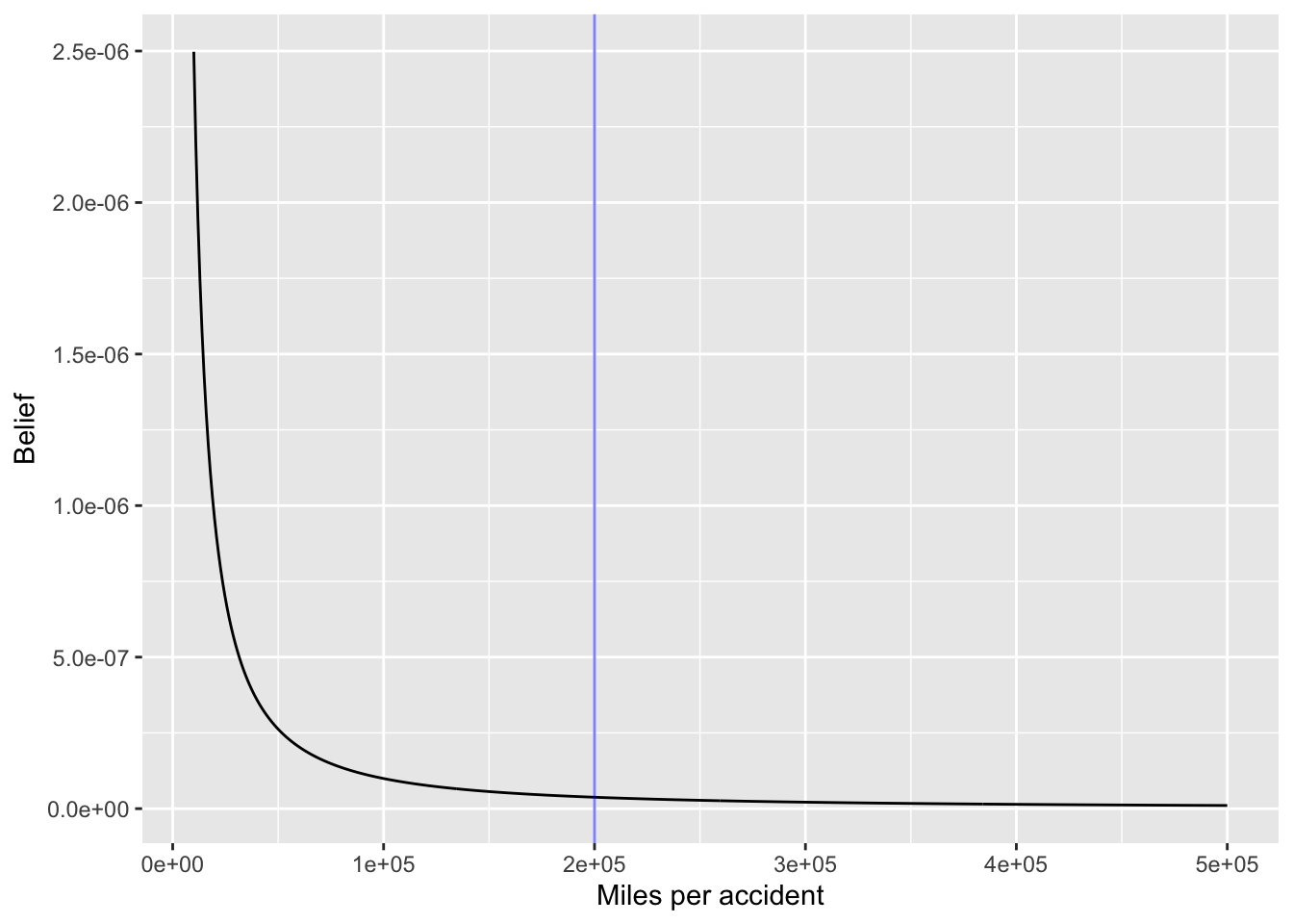
Suppose ordinary new-ish cars have a mean distance between accidents of 200,000 miles. (This is roughly consistent with the Internet factoid that the probability of a car accident in 1000 miles is 1/366.)

What might a skeptical regulator reasonably believe about newly released self-driving cars?

“These things are crazy. Very likely to get in an accident.”

“Perhaps a 1% chance that they are safer than regular cars.”

It takes some math to translate these views into a prediction about the actual mean time between accidents. We teach that in other courses. But here is a graph of such a probability function.

Code

belief <- function(M)  ifelse(M > 1e6 | M < 10, 0, 0.9943/M^1.4)

slice_plot(belief(M=M) ~ M, bounds(M=10000:500000), npts=500) %>%
  gf_vline(xintercept=~ 200000, color="blue", alpha=0.5) %>%
  gf_labs(y="Belief", x="Miles per accident")

This is called a “prior” probability distribution: our starting point.

Now data comes in. Each day we get a report from all the self-driving cars:

• How many miles have they driven successfully, or
• What was their mileage at the crash.

Based on these data, we update our beliefs to produce a “posterior” probability distribution. The Bayesian updating rule is:

Posterior(m) \(\propto\) Likelihood(m, observations) \(\times\) prior(m)

Suppose the observation is: car crashed at 23,241 miles. A plausible **likelihood function* is based on simple probability, not the prior.

Code

crash_likelihood <- function(m, mileage) {
  dexp(mileage, rate=1/m) 
}
slice_plot(crash_likelihood(m, mileage=30000) ~ m, bounds(m=5000:500000)) +
  labs(title="Likelihood function for m given crash at 30,000 miles")

There is also a likelihood function for a car having driven 30,000 miles without an accident.

Code

nocrash_likelihood <- function(m, mileage) {
  (1- pexp(mileage, rate=1/m)) 
}
slice_plot(nocrash_likelihood(m, mileage=30000) ~ m, bounds(m=5000:500000)) +
  labs(title="Likelihood function for m given no crash up to 30,000 miles")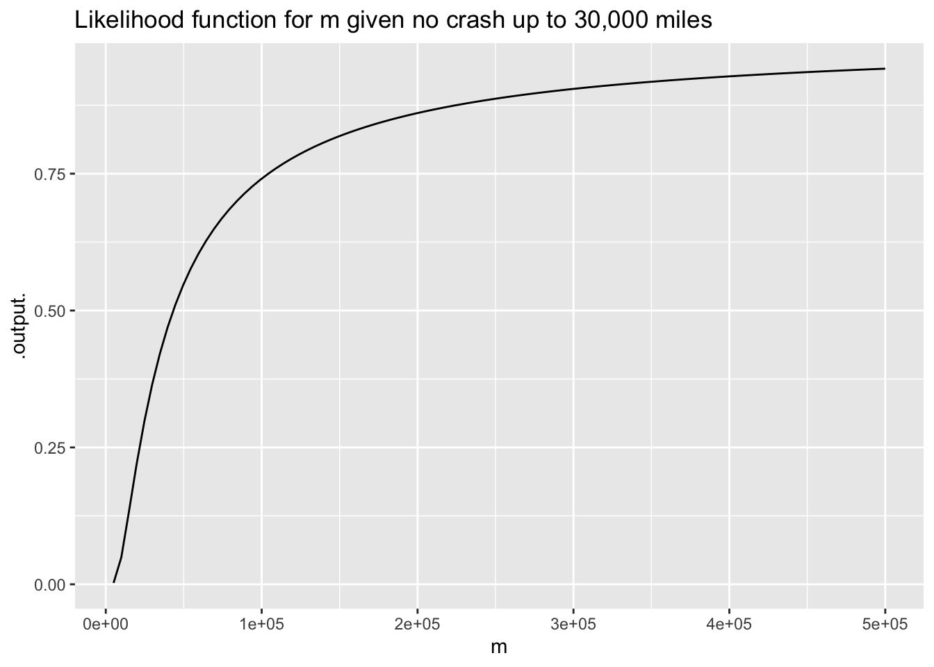

Now for the data

The New York Times report indicates 400 crashes out of 360,000 self-driving cars. Suppose we observe these data for Tesla

95 cars have driven 20K miles without an accident; 5 cars had accidents respectively at 1K, 4K, 8K, 12K, 16K

Code

log_likelihood_observed <- function(m) {
  ( log10(nocrash_likelihood(m, 20000))*95) +
    log10(crash_likelihood(m, 1000)) +
    log10(crash_likelihood(m, 4000)) +
    log10(crash_likelihood(m, 8000)) +
    log10(crash_likelihood(m, 12000)) +
    log10(crash_likelihood(m, 16000)) 
}

Code

log_posterior <- function(m) log_likelihood_observed(m) + log10(belief(m))
slice_plot(10^((log_posterior(m)+38)) ~ m, bounds(m=2000:500000), npts=1001) +
  geom_vline(xintercept=200000, color="red") +
  ylab("Posterior: relative probability") + xlab("Average miles per accident")

The posterior indicates that data on 100 cars, 5 of which had accidents before 20,000 miles, places most belief that the self-driving cars are safer than regular cars: about twice as safe.

This is counter-intuitive, since we have no data on cars that drove farther than 20,000 miles. But would be hard to get 95 out of 100 cars to 20,000 without an accident if the mean distance betwee accidents were even 100,000 miles.